In this post, we demonstrate how to use neural architecture search (NAS) based structural pruning to compress a fine-tuned BERT model to improve model performance and reduce inference times. Pre-trained language models (PLMs) are undergoing rapid commercial and enterprise adoption in the areas of productivity tools, customer service, search and recommendations, business process automation, and content creation. Deploying PLM inference endpoints is typically associated with higher latency and higher infrastructure costs due to the compute requirements and reduced computational efficiency due to the large number of parameters. Pruning a PLM reduces the size and complexity of the model while retaining its predictive capabilities. Pruned PLMs achieve a smaller memory footprint and lower latency. We demonstrate that by pruning a PLM and trading off parameter count and validation error for a specific target task, and are able to achieve faster response times when compared to the base PLM model.

Multi-objective optimization is an area of decision-making that optimizes more than one objective function, such as memory consumption, training time, and compute resources, to be optimized simultaneously. Structural pruning is a technique to reduce the size and computational requirements of PLM by pruning layers or neurons/nodes while attempting to preserve model accuracy. By removing layers, structural pruning achieves higher compression rates, which leads to hardware-friendly structured sparsity that reduces runtimes and response times. Applying a structural pruning technique to a PLM model results in a lighter-weight model with a lower memory footprint that, when hosted as an inference endpoint in SageMaker, offers improved resource efficiency and reduced cost when compared to the original fine-tuned PLM.

The concepts illustrated in this post can be applied to applications that use PLM features, such as recommendation systems, sentiment analysis, and search engines. Specifically, you can use this approach if you have dedicated machine learning (ML) and data science teams who fine-tune their own PLM models using domain-specific datasets and deploy a large number of inference endpoints using Amazon SageMaker. One example is an online retailer who deploys a large number of inference endpoints for text summarization, product catalog classification, and product feedback sentiment classification. Another example might be a healthcare provider who uses PLM inference endpoints for clinical document classification, named entity recognition from medical reports, medical chatbots, and patient risk stratification.

Solution overview

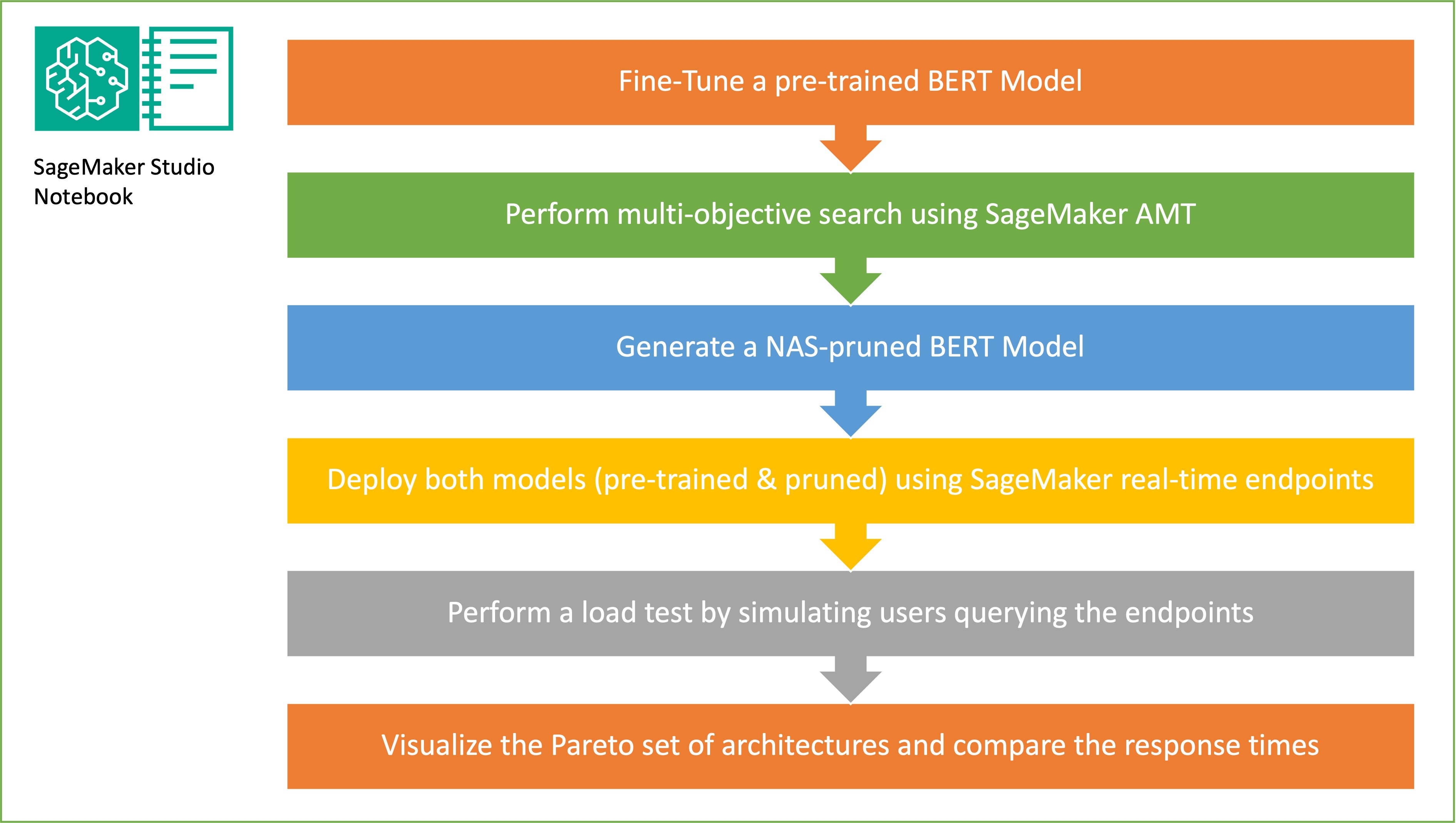
In this section, we present the overall workflow and explain the approach. First, we use an Amazon SageMaker Studio notebook to fine-tune a pre-trained BERT model on a target task using a domain-specific dataset. BERT (Bidirectional Encoder Representations from Transformers) is a pre-trained language model based on the transformer architecture used for natural language processing (NLP) tasks. Neural architecture search (NAS) is an approach for automating the design of artificial neural networks and is closely related to hyperparameter optimization, a widely used approach in the field of machine learning. The goal of NAS is to find the optimal architecture for a given problem by searching over a large set of candidate architectures using techniques such as gradient-free optimization or by optimizing the desired metrics. The performance of the architecture is typically measured using metrics such as validation loss. SageMaker Automatic Model Tuning (AMT) automates the tedious and complex process of finding the optimal combinations of hyperparameters of the ML model that yield the best model performance. AMT uses intelligent search algorithms and iterative evaluations using a range of hyperparameters that you specify. It chooses the hyperparameter values that creates a model that performs the best, as measured by performance metrics such as accuracy and F-1 score.

The fine-tuning approach described in this post is generic and can be applied to any text-based dataset. The task assigned to the BERT PLM can be a text-based task such as sentiment analysis, text classification, or Q&A. In this demo, the target task is a binary classification problem where BERT is used to identify, from a dataset that consists of a collection of pairs of text fragments, whether the meaning of one text fragment can be inferred from the other fragment. We use the Recognizing Textual Entailment dataset from the GLUE benchmarking suite. We perform a multi-objective search using SageMaker AMT to identify the sub-networks that offer optimal trade-offs between parameter count and prediction accuracy for the target task. When performing a multi-objective search, we start with defining the accuracy and parameter count as the objectives that we are aiming to optimize.

Within the BERT PLM network, there can be modular, self-contained sub-networks that allow the model to have specialized capabilities such as language understanding and knowledge representation. BERT PLM uses a multi-headed self-attention sub-network and a feed-forward sub-network. A multi-headed, self-attention layer allows BERT to relate different positions of a single sequence in order to compute a representation of the sequence by allowing multiple heads to attend to multiple context signals. The input is split into multiple subspaces and self-attention is applied to each of the subspaces separately. Multiple heads in a transformer PLM allow the model to jointly attend to information from different representation subspaces. A feed-forward sub-network is a simple neural network that takes the output from the multi-headed self-attention sub-network, processes the data, and returns the final encoder representations.

The goal of random sub-network sampling is to train smaller BERT models that can perform well enough on target tasks. We sample 100 random sub-networks from the fine-tuned base BERT model and evaluate 10 networks simultaneously. The trained sub-networks are evaluated for the objective metrics and the final model is chosen based on the trade-offs found between the objective metrics. We visualize the Pareto front for the sampled sub-networks, which contains the pruned model that offers the optimal trade-off between model accuracy and model size. We select the candidate sub-network (NAS-pruned BERT model) based on the model size and model accuracy that we are willing to trade off. Next, we host the endpoints, the pre-trained BERT base model, and the NAS-pruned BERT model using SageMaker. To perform load testing, we use Locust, an open source load testing tool that you can implement using Python. We run load testing on both endpoints using Locust and visualize the results using the Pareto front to illustrate the trade-off between response times and accuracy for both models. The following diagram provides an overview of the workflow explained in this post.

Prerequisites

For this post, the following prerequisites are required:

You also need to increase the service quota to access at least three instances of ml.g4dn.xlarge instances in SageMaker. The instance type ml.g4dn.xlarge is the cost efficient GPU instance that allows you to run PyTorch natively. To increase the service quota, complete the following steps:

1. On the console, navigate to Service Quotas.
2. For Manage quotas, choose Amazon SageMaker, then choose View quotas.

3. Search for “ml-g4dn.xlarge for training job usage” and select the quota item.
4. Choose Request increase at account-level.

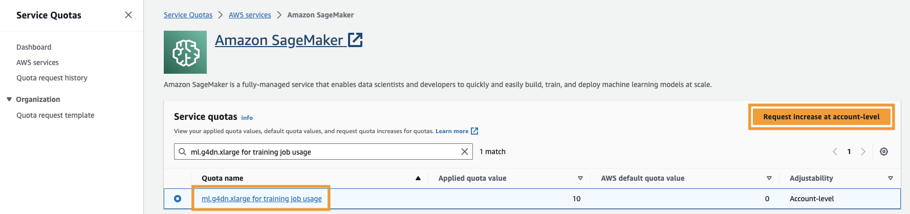
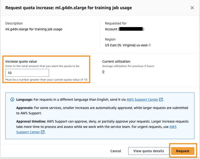
5. For Increase quota value, enter a value of 5 or higher.
6. Choose Request.

The requested quota approval may take some time to complete depending on the account permissions.

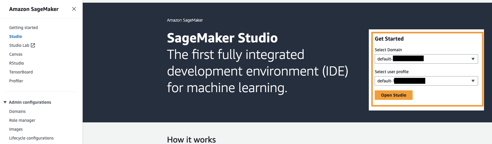
7. Open SageMaker Studio from the SageMaker console.

8. Choose System terminal under Utilities and files.

9. Run the following command to clone the GitHub repo to the SageMaker Studio instance:

   git clone https://github.com/aws/amazon-sagemaker-examples.git

10. Navigate to amazon-sagemaker-examples/hyperparameter_tuning/neural_architecture_search_llm.
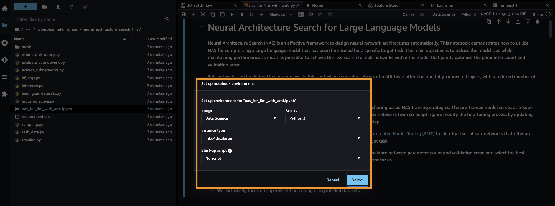
11. Open the file nas_for_llm_with_amt.ipynb.
12. Set up the environment with an ml.g4dn.xlarge instance and choose Select.

Set up the pre-trained BERT model

In this section, we import the Recognizing Textual Entailment dataset from the dataset library and split the dataset into training and validation sets. This dataset consists of pairs of sentences. The task of the BERT PLM is to recognize, given two text fragments, whether the meaning of one text fragment can be inferred from the other fragment. In the following example, we can infer the meaning of the first phrase from the second phrase:

Phrase 1: A man with a beard, wearing a red shirt with gray sleeves and work gloves, pulling on a rope.
Phrase 2: A bearded man pulls a rope

We load the textual recognizing entailment dataset from the GLUE benchmarking suite via the dataset library from Hugging Face within our training script (./training.py). We split the original training dataset from GLUE into a training and validation set. In our approach, we fine-tune the base BERT model using the training dataset, then we perform a multi-objective search to identify the set of sub-networks that optimally balance between the objective metrics. We use the training dataset exclusively for fine-tuning the BERT model. However, we use validation data for the multi-objective search by measuring accuracy on the holdout validation dataset.

Fine-tune the BERT PLM using a domain-specific dataset

The typical use cases for a raw BERT model include next sentence prediction or masked language modeling. To use the base BERT model for downstream tasks such as textual recognizing entailment, we have to further fine-tune the model using a domain-specific dataset. You can use a fine-tuned BERT model for tasks such as sequence classification, question answering, and token classification. However, for the purposes of this demo, we use the fine-tuned model for binary classification. We fine-tune the pre-trained BERT model with the training dataset that we prepared previously, using the following hyperparameters:

hyperparameters["per_device_train_batch_size"] = 8
hyperparameters["per_device_eval_batch_size"] = 8
hyperparameters["learning_rate"] = 2e-05
hyperparameters["num_train_epochs"] = 5
hyperparameters["save_strategy"] = "epoch"
hyperparameters[
"is_regression"
] = False  # set this to True if your dataset is a regression dataset, for example STSB

We save the checkpoint of the model training to an Amazon Simple Storage Service (Amazon S3) bucket, so that the model can be loaded during the NAS-based multi-objective search. Before we train the model, we define the metrics such as epoch, training loss, number of parameters, and validation error:

session = Session()
s3_bucket = session.default_bucket()
s3_bucket_prefix = "nas_amt/model_checkpoint"
s3_path = f"s3://{s3_bucket}/{s3_bucket_prefix}"

metric_definitions = [
    {"Name": "epoch", "Regex": "epoch: ([0-9.]+)"},
    {"Name": "training-loss", "Regex": "training loss: ([0-9.]+)"},
    {"Name": "num-parameters", "Regex": "number of parameters: ([0-9.]+)"},
    {"Name": "validation-error", "Regex": "validation error: ([0-9.]+)"},
]

sm_args = dict(
    entry_point="training.py",
    source_dir=os.path.abspath(""),
    instance_type="ml.g4dn.xlarge",
    instance_count=1,
    py_version="py39",
    framework_version="1.13",
    transformers_version="4.26",
    max_run=3600 * 72,
    role=get_execution_role(),
    checkpoint_local_path="/opt/ml/checkpoints",
    hyperparameters=hyperparameters,
    checkpoint_s3_uri=s3_path,
    metric_definitions=metric_definitions,
)
est = PyTorch(**sm_args)
est.fit()

After the fine-tuning process starts, the training job takes around 15 minutes to complete.

Perform a multi-objective search to select sub-networks and visualize the results

In the next step, we perform a multi-objective search on the fine-tuned base BERT model by sampling random sub-networks using SageMaker AMT. To access a sub-network within the super-network (the fine-tuned BERT model), we mask out all the components of the PLM that are not part of the sub-network. Masking a super-network to find sub-networks in a PLM is a technique used to isolate and identify patterns of the model’s behavior. Note that Hugging Face transformers needs the hidden size to be a multiple of the number of heads. The hidden size in a transformer PLM controls the size of the hidden state vector space, which impacts the model’s ability to learn complex representations and patterns in the data. In a BERT PLM, the hidden state vector is of a fixed size (768). We can’t change the hidden size, and therefore the number of heads has to be in [1, 3, 6, 12].

In contrast to single-objective optimization, in the multi-objective setting, we typically don’t have a single solution that simultaneously optimizes all objectives. Instead, we aim to collect a set of solutions that dominate all other solutions in at least one objective (such as validation error). Now we can start the multi-objective search through AMT by setting the metrics that we want to reduce (validation error and number of parameters). The random sub-networks are defined by the parameter max_jobs and the number of simultaneous jobs is defined by the parameter max_parallel_jobs. The code to load the model checkpoint and evaluate the sub-network is available in the evaluate_subnetwork.py script.

# Maximum number of sub-networks we will evaluate
max_jobs = 100
max_parallel_jobs = 5

# Entry point script to load the super-network and evaluate a sub-network
entry_point = "evaluate_subnetwork.py"

# Command line arguments for the entry point script
hyperparameters = {"model_name_or_path": model_type, "output_dir": "./tmp", "task_name": "rte"}

# Define the metric we want to minimize
metric_definitions = [
    {"Name": "num-parameters", "Regex": "number of parameters: ([0-9.]+)"},
    {"Name": "validation-error", "Regex": "validation error: ([0-9.]+)"},
]

# Define HuggingFace estimator
estimator = HuggingFace(
    entry_point=entry_point,
    source_dir="./",
    instance_type="ml.g4dn.xlarge",  # instance types for the SageMaker training jobs
    instance_count=1,
    py_version="py39",
    framework_version="1.13",
    pytorch_version="1.13",
    transformers_version="4.26",
    max_run=3600 * 72,
    role=get_execution_role(),
    volume_size=125,
    model_uri=s3_path,
    hyperparameters=hyperparameters,
)

current_time = datetime.now().strftime("%m-%d-%Y-%H-%M-%S")
tuning_job_name = f"nas-search-{current_time}"

# Search space to define sub-networks
hyperparameter_ranges = {
    "num_layers": IntegerParameter(0, 12),
    # To meet HuggingFace constraints, we can only set the number of head to these values
    "num_heads": CategoricalParameter([1, 3, 6, 12]),
    "num_units": IntegerParameter(0, 3072),
}

# Define AMT Tuner object
my_tuner = HyperparameterTuner(
    estimator=estimator,
    objective_metric_name="validation-error",
    hyperparameter_ranges=hyperparameter_ranges,
    metric_definitions=metric_definitions,
    max_jobs=max_jobs,
    strategy="Random",
    random_seed=seed,
    objective_type="Minimize",
    max_parallel_jobs=max_parallel_jobs,
)

# Start hyperparameter tuning job
my_tuner.fit(job_name=tuning_job_name)

The AMT tuning job takes approximately 2 hours and 20 minutes to run. After the AMT tuning job runs successfully, we parse the job’s history and collect the sub-network’s configurations, such as number of heads, number of layers, number of units, and the corresponding metrics such as validation error and number of parameters. The following screenshot shows the summary of a successful AMT tuner job.

Next, we visualize the results using a Pareto set (also known as Pareto frontier or Pareto optimal set), which helps us identify optimal sets of sub-networks that dominate all other sub-networks in the objective metric (validation error):

history = my_tuner.analytics().dataframe()
data = []
configs = []
for i, t in enumerate(my_tuner.analytics().training_job_summaries()):
    jn = t["TrainingJobName"]
    df = sagemaker.analytics.TrainingJobAnalytics(jn).dataframe()

    row = history[history["TrainingJobName"] == jn]
    config = {
        "num-heads": int(row["num_heads"].iloc[0].strip('"')),
        "num-layers": int(row["num_layers"]),
        "num-units": int(row["num_units"]),
    }
    configs.append(config)

    p = []
    for j, metric in enumerate(metric_definitions):
        metric_name = metric["Name"]
        if "metric_name" not in df.keys():
            continue
        y = float(df[df["metric_name"] == metric_name]["value"])
        p.append(y)
    if len(p) > 0:
        data.append(p)

data = np.array(data)

First, we collect the data from the AMT tuning job. Then then we plot the Pareto set using matplotlob.pyplot with number of parameters in the x axis and validation error in the y axis. This implies that when we move from one sub-network of the Pareto set to another, we must either sacrifice performance or model size but improve the other. Ultimately, the Pareto set provides us the flexibility to choose the sub-network that best suits our preferences. We can decide how much we want to reduce the size of our network and how much performance we are willing to sacrifice.

import matplotlib.pyplot as plt
from multi_objective import get_pareto_optimal

# get results of the un-pruned network
df = sagemaker.analytics.TrainingJobAnalytics(est.jobs[0].name).dataframe()
validation_error_unpruned_network = float(df[df["metric_name"] == "validation-error"].value.min())
params_unpruned_network = int(df[df["metric_name"] == "num-parameters"].value.min())
plt.scatter(
params_unpruned_network,
validation_error_unpruned_network,
marker="o",
s=80,
facecolors="none",
edgecolors="C3",
linewidth=2,
label="un-pruned super-network",
)
# get Pareto optimal points
idx = get_pareto_optimal(data)
x = data[idx, 0]
y = data[idx, 1]
plt.scatter(
x,
y,
marker="o",
s=80,
facecolors="none",
edgecolors="C0",
linewidth=2,
label="Pareto front (sub-networks)",
)
plt.xlabel("number of parameters")
plt.ylabel("validation error")
plt.legend()
plt.xscale("log")
plt.grid(linewidth="1", alpha=0.4, which="both")

Deploy the fine-tuned BERT model and the NAS-optimized sub-network model using SageMaker

Next, we deploy the largest model in our Pareto set that leads to the smallest amount of performance degeneration to a SageMaker endpoint. The best model is the one that provides an optimal trade-off between the validation error and the number of parameters for our use case.

# Let's take the largest model in the Pareto set
indicies = np.arange(len(configs))[idx]
pareto_optimal_sub_networks = [configs[i] for i in indicies]
config_to_deploy = pareto_optimal_sub_networks[-1]  

from sagemaker.huggingface.model import HuggingFaceModel

# create Hugging Face Model Class
huggingface_model = HuggingFaceModel(
    model_data=s3_path + "/model.tar.gz",
    role=get_execution_role(),
    transformers_version="4.26",
    pytorch_version="1.13",
    py_version="py39",
    entry_point="inference.py",
    source_dir="./",
    env={"SM_HPS": json.dumps(config_to_deploy)},
)

# deploy model to SageMaker Inference
predictor = huggingface_model.deploy(initial_instance_count=1, instance_type="ml.g4dn.xlarge")

Model comparison

We took a pre-trained base BERT model, fine-tuned it using a domain-specific dataset, ran a NAS search to identify dominant sub-networks based on the objective metrics, and deployed the pruned model on a SageMaker endpoint. In addition, we took the pre-trained base BERT model and deployed the base model on a second SageMaker endpoint. Next, we ran load-testing using Locust on both inference endpoints and evaluated the performance in terms of response time.

First, we import the necessary Locust and Boto3 libraries. Then we construct a request metadata and record the start time to be used for load testing. Then the payload is passed to the SageMaker endpoint invoke API via the BotoClient to simulate real user requests. We use Locust to spawn multiple virtual users to send requests in parallel and measure the endpoint performance under the load. Tests are run by increasing the number of users for each of the two endpoints, respectively. After the tests are completed, Locust outputs a request statistics CSV file for each of the deployed models.

def send(self):
        request_meta = {
            "request_type": "InvokeEndpoint",
            "name": "SageMaker",
            "start_time": time.time(),
            "response_length": 0,
            "response": None,
            "context": {},
            "exception": None,
        }
        start_perf_counter = time.perf_counter()

        try:
            response = self.sagemaker_client.invoke_endpoint(
                EndpointName=self.endpoint_name,
                Body=self.payload,
                ContentType=self.content_type,
            )
            logging.info(response["Body"].read())
        except Exception as e:
            request_meta["exception"] = e

        request_meta["response_time"] = (
            time.perf_counter() - start_perf_counter
        ) * 1000

        events.request.fire(**request_meta)

Next, we generate the response time plots from the CSV files downloaded after running the tests with Locust. The purpose of plotting the response time vs. the number of users is to analyze the load testing results by visualizing the impact of the response time of the model endpoints. In the following chart, we can see that the NAS-pruned model endpoint achieves a lower response time compared to the base BERT model endpoint.

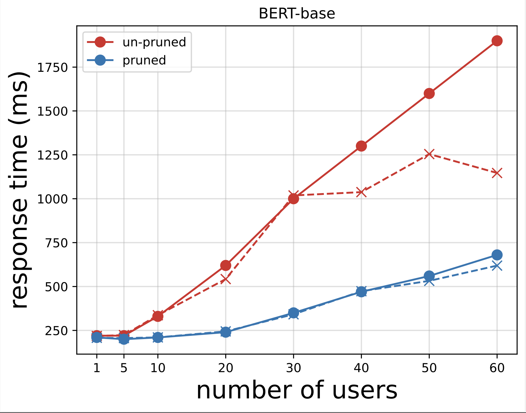
In the second chart, which is an extension of the first chart, we observe that after around 70 users, SageMaker starts to throttle the base BERT model endpoint and throws an exception. However, for the NAS-pruned model endpoint, the throttling happens between 90–100 users and with a lower response time.

From the two charts, we observe that the pruned model has a faster response time and scales better when compared to the unpruned model. As we scale the number of inference endpoints, as is the case with users who deploy a large number of inference endpoints for their PLM applications, the cost benefits and performance improvement start to become quite substantial.

Clean up

To delete the SageMaker endpoints for the fine-tuned base BERT model and the NAS-pruned model, complete the following steps:

1. On the SageMaker console, choose Inference and Endpoints in the navigation pane.
2. Select the endpoint and delete it.

Alternatively, from the SageMaker Studio notebook, run the following commands by providing the endpoint names:

predictor.delete_model()
predictor.delete_endpoint()

Conclusion

In this post, we discussed how to use NAS to prune a fine-tuned BERT model. We first trained a base BERT model using domain-specific data and deployed it to a SageMaker endpoint. We performed a multi-objective search on the fine-tuned base BERT model using SageMaker AMT for a target task. We visualized the Pareto front and selected the Pareto optimal NAS-pruned BERT model and deployed the model to a second SageMaker endpoint. We performed load testing using Locust to simulate users querying both the endpoints, and measured and recorded the response times in a CSV file. We plotted the response time vs. the number of users for both the models.

We observed that the pruned BERT model performed significantly better in both response time and instance throttling threshold. We concluded that the NAS-pruned model was more resilient to an increased load on the endpoint, maintaining a lower response time even as more users stressed the system compared to the base BERT model. You can apply the NAS technique described in this post to any large language model to find a pruned model that can perform the target task with significantly lower response time. You can further optimize the approach by using latency as a parameter in addition to validation loss.

Although we use NAS in this post, quantization is another common approach used to optimize and compress PLM models. Quantization reduces the precision of the weights and activations in a trained network from 32-bit floating point to lower bit widths such as 8-bit or 16-bit integers, which results in a compressed model that generates faster inference. Quantization doesn’t reduce the number of parameters; instead it reduces the precision of the existing parameters to get a compressed model. NAS pruning removes redundant networks in a PLM, which creates a sparse model with fewer parameters. Typically, NAS pruning and quantization are used together to compress large PLMs to maintain model accuracy, reduce validation losses while improving performance, and reduce model size. The other commonly used techniques to reduce the size of PLMs include knowledge distillation, matrix factorization, and distillation cascades.

The approach proposed in the blogpost is suitable for teams that use SageMaker to train and fine-tune the models using domain-specific data and deploy the endpoints to generate inference. If you’re looking for a fully managed service that offers a choice of high-performing foundation models needed to build generative AI applications, consider using Amazon Bedrock. If you’re looking for pre-trained, open source models for a wide range of business use cases and want to access solution templates and example notebooks, consider using Amazon SageMaker JumpStart. A pre-trained version of the Hugging Face BERT base cased model that we used in this post is also available from SageMaker JumpStart.

About the Authors

Aparajithan Vaidyanathan is a Principal Enterprise Solutions Architect at AWS. He is a Cloud Architect with 24+ years of experience designing and developing enterprise, large-scale and distributed software systems. He specializes in Generative AI and Machine Learning Data Engineering. He is an aspiring marathon runner and his hobbies include hiking, bike riding and spending time with his wife and two boys.

Aaron Klein is a Sr Applied Scientist at AWS working on automated machine learning methods for deep neural networks.

Jacek Golebiowski is a Sr Applied Scientist at AWS.

• SEO Powered Content & PR Distribution. Get Amplified Today.
• PlatoData.Network Vertical Generative Ai. Empower Yourself. Access Here.
• PlatoAiStream. Web3 Intelligence. Knowledge Amplified. Access Here.
• PlatoESG. Carbon, CleanTech, Energy, Environment, Solar, Waste Management. Access Here.
• PlatoHealth. Biotech and Clinical Trials Intelligence. Access Here.
• Source: https://aws.amazon.com/blogs/machine-learning/reduce-inference-time-for-bert-models-using-neural-architecture-search-and-sagemaker-automated-model-tuning/