Image by pch.vector on Freepik
 

Hi everyone! I am sure you are reading this article because you are interested in a machine-learning model and want to build one.

You may have tried to develop machine learning models before or you are entirely new to the concept. No matter your experience, this article will guide you through the best practices for developing machine learning models.

In this article, we will develop a Customer Churn prediction classification model following the steps below:

1. Business Understanding
2. Data Collection and Preparation

• Collecting Data
• Exploratory Data Analysis (EDA) and Data Cleaning
• Feature Selection

3. Building the Machine Learning Model

• Choosing the Right Model
• Splitting the Data
• Training the Model
• Model Evaluation

4. Model Optimization

5. Deploying the Model

Let’s get into it if you are excited about building your first machine learning model.

Understanding the Basics

 
Before we get into the machine learning model development, let’s briefly explain machine learning, the types of machine learning, and a few terminologies we will use in this article.

First, let’s discuss the types of machine learning models we can develop. Four main types of Machine Learning often developed are:

• Supervised Machine Learning is a machine learning algorithm that learns from labeled datasets. Based on the correct output, the model learns from the pattern and tries to predict the new data. There are two categories in Supervised Machine Learning: Classification (Category prediction) and Regression (Numerical prediction).
• Unsupervised Machine Learning is an algorithm that tries to find patterns in data without direction. Unlike supervised machine learning, the model is not guided by label data. This type has two common categories: Clustering (Data Segmentation) and Dimensionality Reduction (Feature Reduction).
• Semi-supervised machine learning combines the labeled and unlabeled datasets, where the labeled dataset guides the model in identifying patterns in the unlabeled data. The simplest example is a self-training model that can label the unlabeled data based on a labeled data pattern.
• Reinforcement Learning is a machine learning algorithm that can interact with the environment and react based on the action (getting a reward or punishment). It would maximize the result with the rewards system and avoid bad results with punishment. An example of this model application is the self-driving car.

You also need to know a few terminologies to develop a machine-learning model:

• Features: Input variables used to make predictions in a machine learning model.
• Labels: Output variables that the model is trying to predict.
• Data Splitting: The process of data separation into different sets.
• Training Set: Data used to train the machine learning model.
• Test Set: Data used to evaluate the performance of the trained model.
• Validation Set: Data use used during the training process to tune hyperparameters
• Exploratory Data Analysis (EDA): The process of analyzing and visualizing datasets to summarize their information and discover patterns.
• Models: The outcome of the Machine Learning process. They are the mathematical representation of the patterns and relationships within the data.
• Overfitting: Occurs when the model is generalized too well and learns the data noise. The model can predict well in the training but not in the test set.
• Underfitting: When a model is too simple to capture the underlying patterns in the data. The model performance in training and test sets could be better.
• Hyperparameters: Configuration settings are used to tune the model and are set before training begins.
• Cross-validation: a technique for evaluating the model by partitioning the original sample into training and validation sets multiple times.
• Feature Engineering: Using domain knowledge to get new features from raw data.
• Model Training: The process of learning the parameters of a model using the training data.
• Model Evaluation: Assessing the performance of a trained model using machine learning metrics like accuracy, precision, and recall.
• Model Deployment: Making a trained model available in a production environment.

With all this basic knowledge, let’s learn to develop our first machine-learning model.
 

1. Business Understanding

 
Before any machine learning model development, we must understand why we must develop the model. That’s why understanding what the business wants is necessary to ensure the model is valid.
Business understanding usually requires a proper discussion with the related stakeholders. Still, since this tutorial does not have business users for the machine learning model, we assume the business needs ourselves.

As stated previously, we would develop a Customer Churn prediction model. In this case, the business needs to avoid further churn from the company and wants to take action for the customer with a high probability of churning.
With the above business requirements, we need specific metrics to measure whether the model performs well. There are many measurements, but I propose using the Recall metric.

In monetary values, it might be more beneficial to use Recall, as it tries to minimize the False Negative or decrease the amount of prediction that was not churning while it’s churning. Of course, we can try to aim for balance by using the F1 metric.

With that in mind, let’s get into the first part of our tutorial.
 

2. Data Collection and Preparation

Data Collection

Data is the heart of any machine learning project. Without it, we can’t have a machine learning model to train. That’s why we need quality data with proper preparation before we input them into the machine learning algorithm.

In a real-world case, clean data does not come easily. Often, we need to collect it through applications, surveys, and many other sources before storing it in data storage. However, this tutorial only covers collecting the dataset as we use the existing clean data.

In our case, we would use the Telco Customer Churn data from the Kaggle. It’s open-source classification data regarding customer history in the telco industry with the churn label.
 

Exploratory Data Analysis (EDA) and Data Cleaning

 
Let’s start by reviewing our dataset. I assume the reader already has basic Python knowledge and can use Python packages in their notebook. I also based the tutorial on Anaconda environment distribution to make things easier.

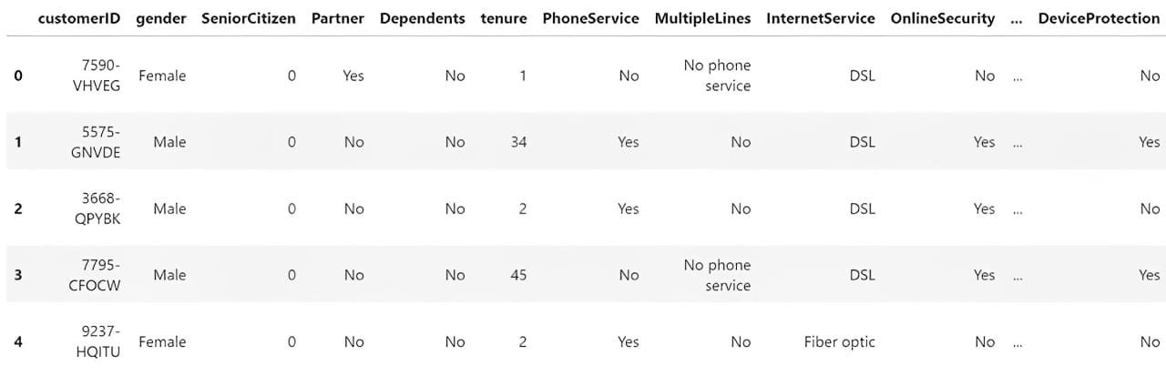
To understand the data we have, we need to load it into a Python package for data manipulation. The most famous one is the Pandas Python package, which we will use. We can use the following code to load and review the CSV data.

import pandas as pd

df = pd.read_csv('WA_Fn-UseC_-Telco-Customer-Churn.csv')
df.head()

Next, we would explore the data to understand our dataset. Here are a few actions that we would perform for the EDA process.

1. Examining the features and the summary statistics.
2. Checks for missing values in the features.
3. Analyze the distribution of the label (Churn).
4. Plots histograms for numerical features and bar plots for categorical features.
5. Plots a correlation heatmap for numerical features.
6. Uses box plots to identify distributions and potential outliers.

First, we would check the features and summary statistics. With Pandas, we can see our dataset features using the following code.

# Get the basic information about the dataset
df.info()

Output>>

RangeIndex: 7043 entries, 0 to 7042
Data columns (total 21 columns):
 #   Column            Non-Null Count  Dtype  
---  ------            --------------  -----  
 0   customerID        7043 non-null   object 
 1   gender            7043 non-null   object 
 2   SeniorCitizen     7043 non-null   int64  
 3   Partner           7043 non-null   object 
 4   Dependents        7043 non-null   object 
 5   tenure            7043 non-null   int64  
 6   PhoneService      7043 non-null   object 
 7   MultipleLines     7043 non-null   object 
 8   InternetService   7043 non-null   object 
 9   OnlineSecurity    7043 non-null   object 
 10  OnlineBackup      7043 non-null   object 
 11  DeviceProtection  7043 non-null   object 
 12  TechSupport       7043 non-null   object 
 13  StreamingTV       7043 non-null   object 
 14  StreamingMovies   7043 non-null   object 
 15  Contract          7043 non-null   object 
 16  PaperlessBilling  7043 non-null   object 
 17  PaymentMethod     7043 non-null   object 
 18  MonthlyCharges    7043 non-null   float64
 19  TotalCharges      7043 non-null   object 
 20  Churn             7043 non-null   object 
dtypes: float64(1), int64(2), object(18)
memory usage: 1.1+ MB

We would also get the dataset summary statistics with the following code.

# Get the numerical summary statistics of the dataset
df.describe()

# Get the categorical summary statistics of the dataset
df.describe(exclude = 'number')

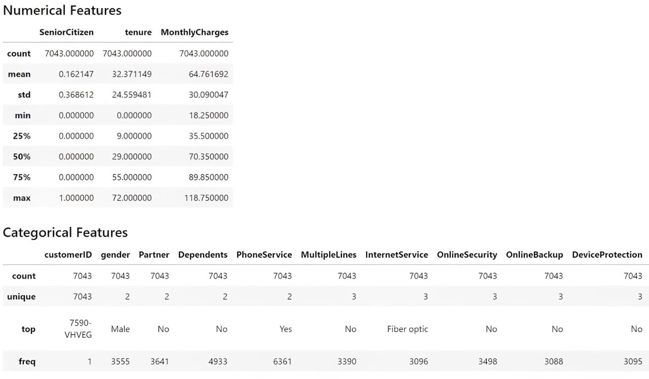
From the information above, we understand that we have 19 features with one target feature (Churn). The dataset contains 7043 rows, and most datasets are categorical.

Let’s check for the missing data.

# Check for missing values
print(df.isnull().sum())

Output>>
Missing Values:
customerID          0
gender              0
SeniorCitizen       0
Partner             0
Dependents          0
tenure              0
PhoneService        0
MultipleLines       0
InternetService     0
OnlineSecurity      0
OnlineBackup        0
DeviceProtection    0
TechSupport         0
StreamingTV         0
StreamingMovies     0
Contract            0
PaperlessBilling    0
PaymentMethod       0
MonthlyCharges      0
TotalCharges        0
Churn               0

Our dataset does not contain missing data, so we don’t need to perform any missing data treatment activity.
Then, we would check the target variable to see if we have an imbalance case.

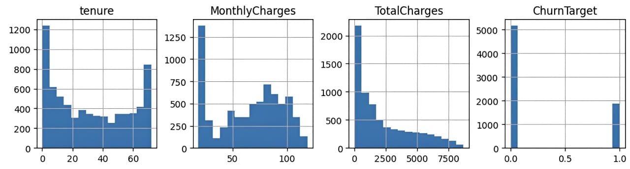
print(df['Churn'].value_counts())

Output>>
Distribution of Target Variable:
No     5174
Yes    1869

There is a slight imbalance, as only close to 25% of the churn occurs compared to the non-churn cases.

Let’s also see the distribution of the other features, starting with the numerical features. However, we would also transform the TotalCharges feature into a numerical column, as this feature should be numerical rather than a category. Additionally, the SeniorCitizen feature should be categorical so that I would transform it into strings. Also, as the Churn feature is categorical, we would develop new features that show it as a numerical column.

import numpy as np
df['TotalCharges'] = df['TotalCharges'].replace('', np.nan)
df['TotalCharges'] = pd.to_numeric(df['TotalCharges'], errors='coerce').fillna(0)

df['SeniorCitizen'] = df['SeniorCitizen'].astype('str')

df['ChurnTarget'] = df['Churn'].apply(lambda x: 1 if x=='Yes' else 0)

df['ChurnTarget'] = df['Churn'].apply(lambda x: 1 if x=='Yes' else 0)

num_features = df.select_dtypes('number').columns
df[num_features].hist(bins=15, figsize=(15, 6), layout=(2, 5))

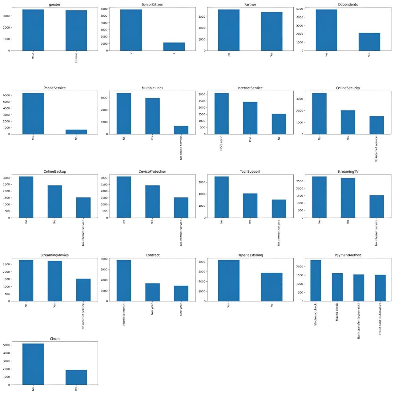
We would also provide categorical feature plotting except for the customerID, as they are identifiers with unique values.

import matplotlib.pyplot as plt
# Plot distribution of categorical features
cat_features = df.drop('customerID', axis =1).select_dtypes(include='object').columns

plt.figure(figsize=(20, 20))
for i, col in enumerate(cat_features, 1):
    plt.subplot(5, 4, i)
    df[col].value_counts().plot(kind='bar')
    plt.title(col)

We then would see the correlation between numerical features with the following code.

import seaborn as sns

# Plot correlations between numerical features
plt.figure(figsize=(10, 8))
sns.heatmap(df[num_features].corr())
plt.title('Correlation Heatmap')

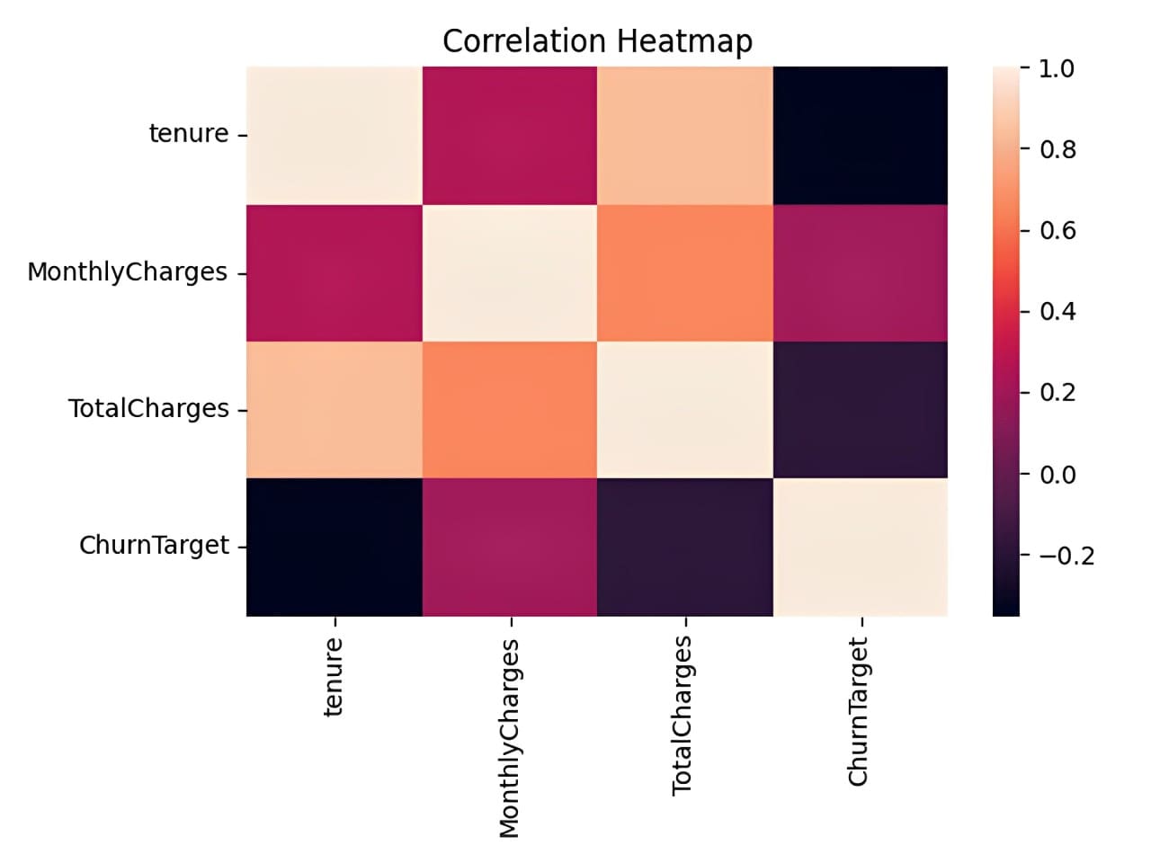
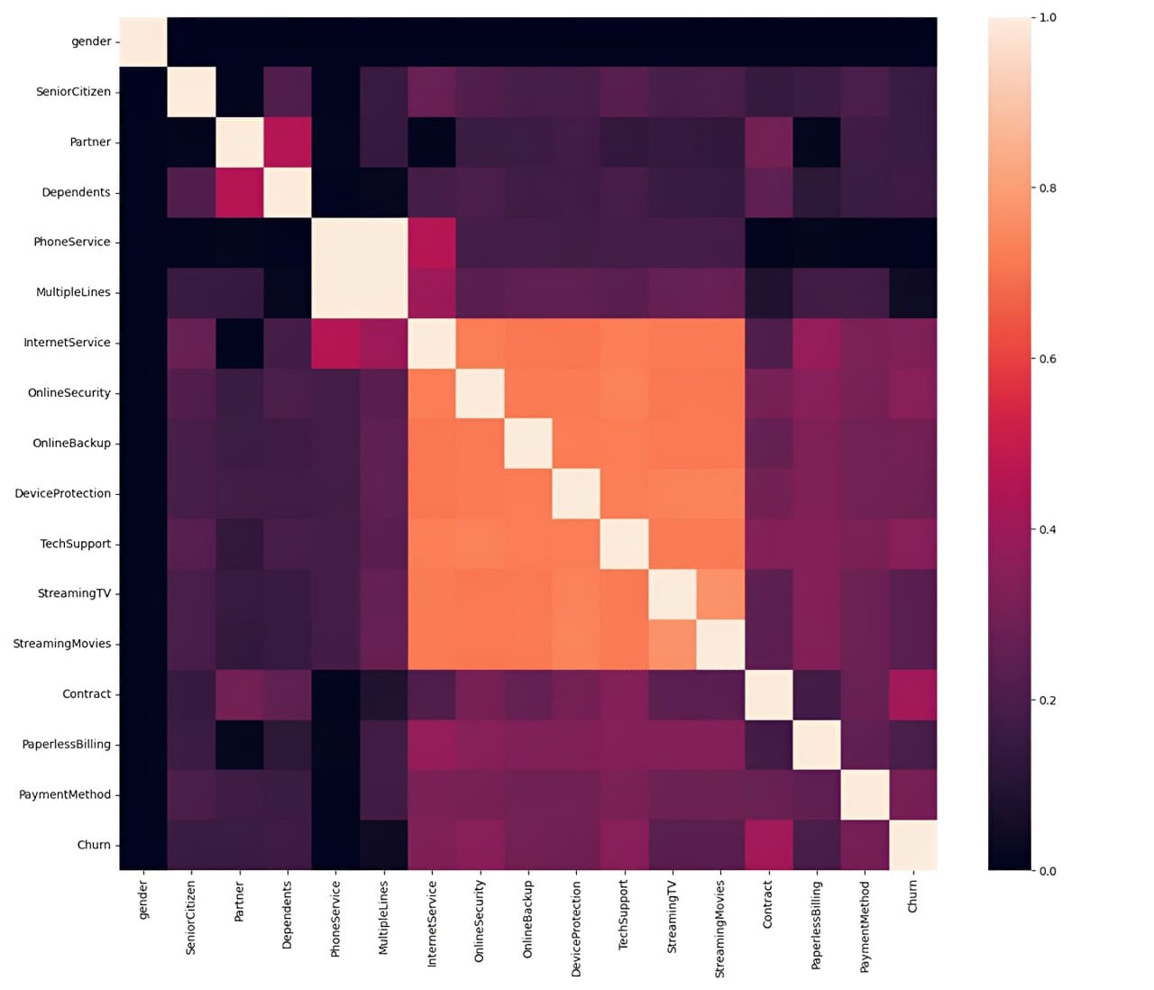
The correlation above is based on the Pearson Correlation, a linear correlation between one feature and the other. We can also perform correlation analysis to categorical analysis with Cramer’s V. To make the analysis easier, we would install Dython Python package that could help our analysis.

pip install dython

Once the package is installed, we will perform the correlation analysis with the following code.

from dython.nominal import associations

# Calculate the Cramer’s V and correlation matrix
assoc = associations(df[cat_features], nominal_columns='all', plot=False)
corr_matrix = assoc['corr']

# Plot the heatmap
plt.figure(figsize=(14, 12))
sns.heatmap(corr_matrix)

Lastly, we would check the numerical outlier with a box plot based on the Interquartile Range (IQR).

# Plot box plots to identify outliers
plt.figure(figsize=(20, 15))
for i, col in enumerate(num_features, 1):
    plt.subplot(4, 4, i)
    sns.boxplot(y=df[col])
    plt.title(col)

From the analysis above, we can see that we should address no missing data or outliers. The next step is to perform feature selection for our machine learning model, as we only want the features that impact the prediction and are viable in the business.

Feature Selection

There are many ways to perform feature selection, usually done by combining business knowledge and technical application. However, this tutorial will only use the correlation analysis we have done previously to make the feature selection.

First, let’s select the numerical features based on the correlation analysis.

target = 'ChurnTarget'
num_features = df.select_dtypes(include=[np.number]).columns.drop(target)

# Calculate correlations
correlations = df[num_features].corrwith(df[target])

# Set a threshold for feature selection
threshold = 0.3
selected_num_features = correlations[abs(correlations) > threshold].index.tolist()

You can play around with the threshold later to see if the feature selection affects the model’s performance. We would also perform the feature selection into the categorical features.

categorical_target = 'Churn'

assoc = associations(df[cat_features], nominal_columns='all', plot=False)
corr_matrix = assoc['corr']

threshold = 0.3
selected_cat_features = corr_matrix[corr_matrix.loc[categorical_target] > threshold ].index.tolist()

del selected_cat_features[-1]

Then, we would combine all the selected features with the following code.

selected_features = []
selected_features.extend(selected_num_features)
selected_features.extend(selected_cat_features)

print(selected_features)

Output>>
['tenure',
 'InternetService',
 'OnlineSecurity',
 'TechSupport',
 'Contract',
 'PaymentMethod']

In the end, we have six features that would be used to develop the customer churn machine learning model.
 

3. Building the Machine Learning Model

Choosing the Right Model

There are many considerations to choosing a suitable model for machine learning development, but it always depends on the business needs. A few points to remember:

1. The use case problem. Is it supervised or unsupervised, or is it classification or regression? Is it Multiclass or Multilabel? The case problem would dictate which model can be used.
2. The data characteristics. Is it tabular data, text, or image? Is the dataset size big or small? Did the dataset contain missing values? Depending on the dataset, the model we choose could be different.
3. How easy is the model to be interpreted? Balancing interpretability and performance is essential for the business.

As a thumb rule, starting with a simpler model as a benchmark is often best before proceeding to a complex one. You can read my previous article about the simple model to understand what constitutes a simple model.

For this tutorial, let’s start with linear model Logistic Regression for the model development.
 

Splitting the Data

The next activity is to split the data into training, test, and validation sets. The purpose of data splitting during machine learning model training is to have a data set that acts as unseen data (real-world data) to evaluate the model unbias without any data leakage.

To split the data, we will use the following code:

from sklearn.model_selection import train_test_split

target = 'ChurnTarget' 

X = df[selected_features]
y = df[target]

cat_features = X.select_dtypes(include=['object']).columns.tolist()
num_features = X.select_dtypes(include=['number']).columns.tolist()

#Splitting data into Train, Validation, and Test Set
X_train_val, X_test, y_train_val, y_test = train_test_split(X, y, test_size=0.2, random_state=42, stratify=y)

X_train, X_val, y_train, y_val = train_test_split(X_train_val, y_train_val, test_size=0.25, random_state=42, stratify=y_train_val)

In the above code, we split the data into 60% of the training dataset and 20% of the test and validation set. Once we have the dataset, we will train the model.
 

Training the Model

As mentioned, we would train a Logistic Regression model with our training data. However, the model can only accept numerical data, so we must preprocess the dataset. This means we need to transform the categorical data into numerical data.

For best practice, we also use the Scikit-Learn pipeline to contain all the preprocessing and modeling steps. The following code allows you to do that.

from sklearn.compose import ColumnTransformer
from sklearn.pipeline import Pipeline
from sklearn.preprocessing import OneHotEncoder
from sklearn.linear_model import LogisticRegression
# Prepare the preprocessing step
preprocessor = ColumnTransformer(
    transformers=[
        ('num', 'passthrough', num_features),
        ('cat', OneHotEncoder(), cat_features)
    ])

pipeline = Pipeline(steps=[
    ('preprocessor', preprocessor),
    ('classifier', LogisticRegression(max_iter=1000))
])

# Train the logistic regression model
pipeline.fit(X_train, y_train)

The model pipeline would look like the image below.

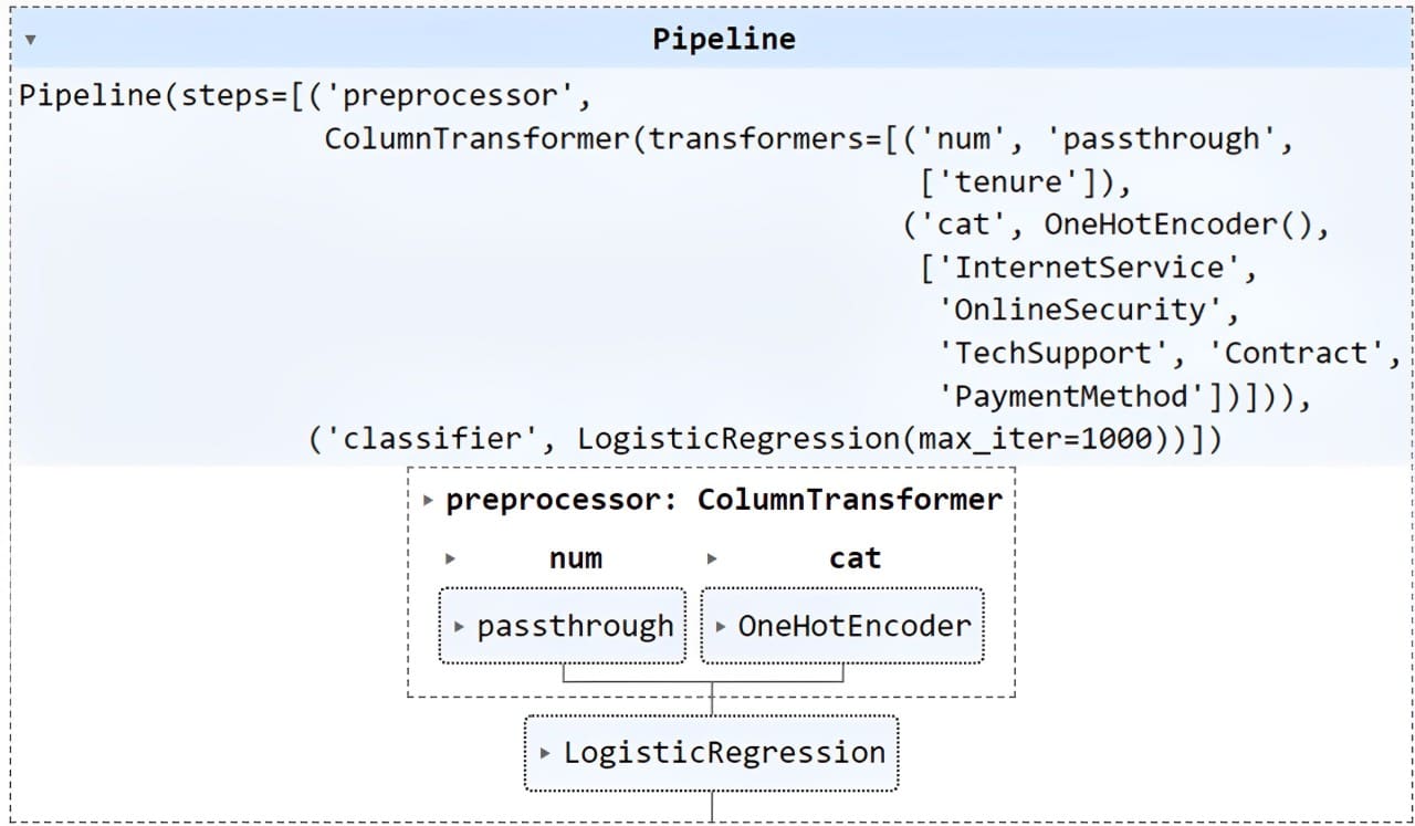
The Scikit-Learn pipeline would accept the unseen data and go through all the preprocessing steps before entering the model. After the model is finished training, let’s evaluate our model result.
 

Model Evaluation

As mentioned, we will evaluate the model by focusing on the Recall metrics. However, the following code shows all the basic classification metrics.

from sklearn.metrics import classification_report

# Evaluate on the validation set
y_val_pred = pipeline.predict(X_val)
print("Validation Classification Report:n", classification_report(y_val, y_val_pred))

# Evaluate on the test set
y_test_pred = pipeline.predict(X_test)
print("Test Classification Report:n", classification_report(y_test, y_test_pred))

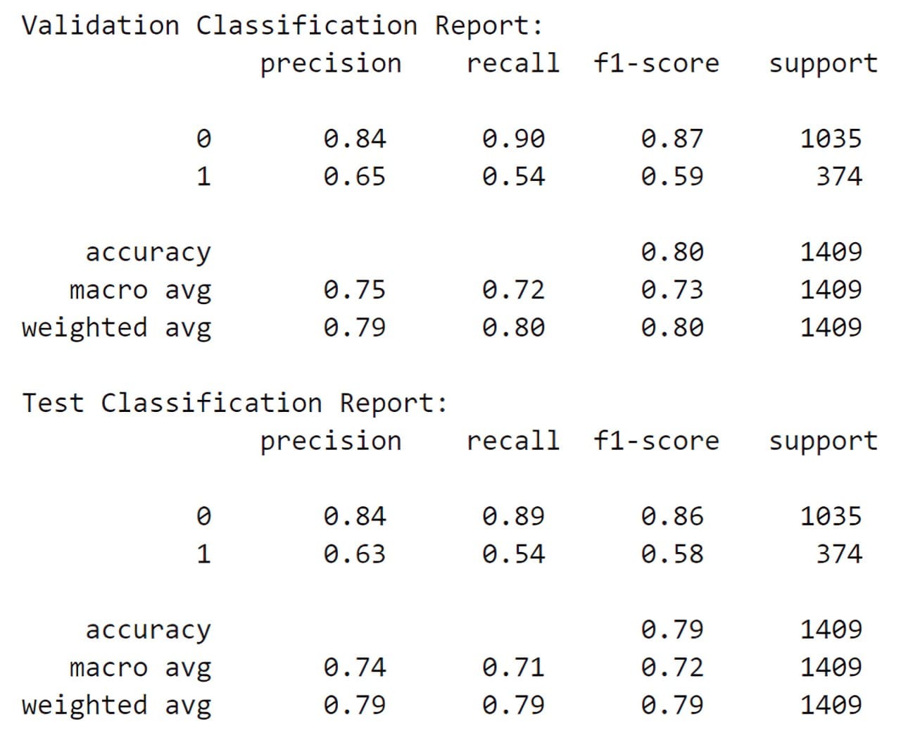
As we can see from the Validation and Test data, the Recall for churn (1) is not the best. That’s why we can optimize the model to get the best result.
 

4. Model Optimization

 
We always need to focus on the data to get the best result. However, optimizing the model could also lead to better results. This is why we can optimize our model. One way to optimize the model is via hyperparameter optimization, which tests all combinations of these model hyperparameters to find the best one based on the metrics.

Every model has a set of hyperparameters we can set before training it. We call hyperparameter optimization the experiment to see which combination is the best. To do that, we can use the following code.

from sklearn.model_selection import GridSearchCV
# Define the logistic regression model within a pipeline
pipeline = Pipeline(steps=[
    ('preprocessor', preprocessor),
    ('classifier', LogisticRegression(max_iter=1000))
])

# Define the hyperparameters for GridSearchCV
param_grid = {
    'classifier__C': [0.1, 1, 10, 100],
    'classifier__solver': ['lbfgs', 'liblinear']
}

# Perform Grid Search with cross-validation
grid_search = GridSearchCV(pipeline, param_grid, cv=5, scoring='recall')
grid_search.fit(X_train, y_train)

# Best hyperparameters
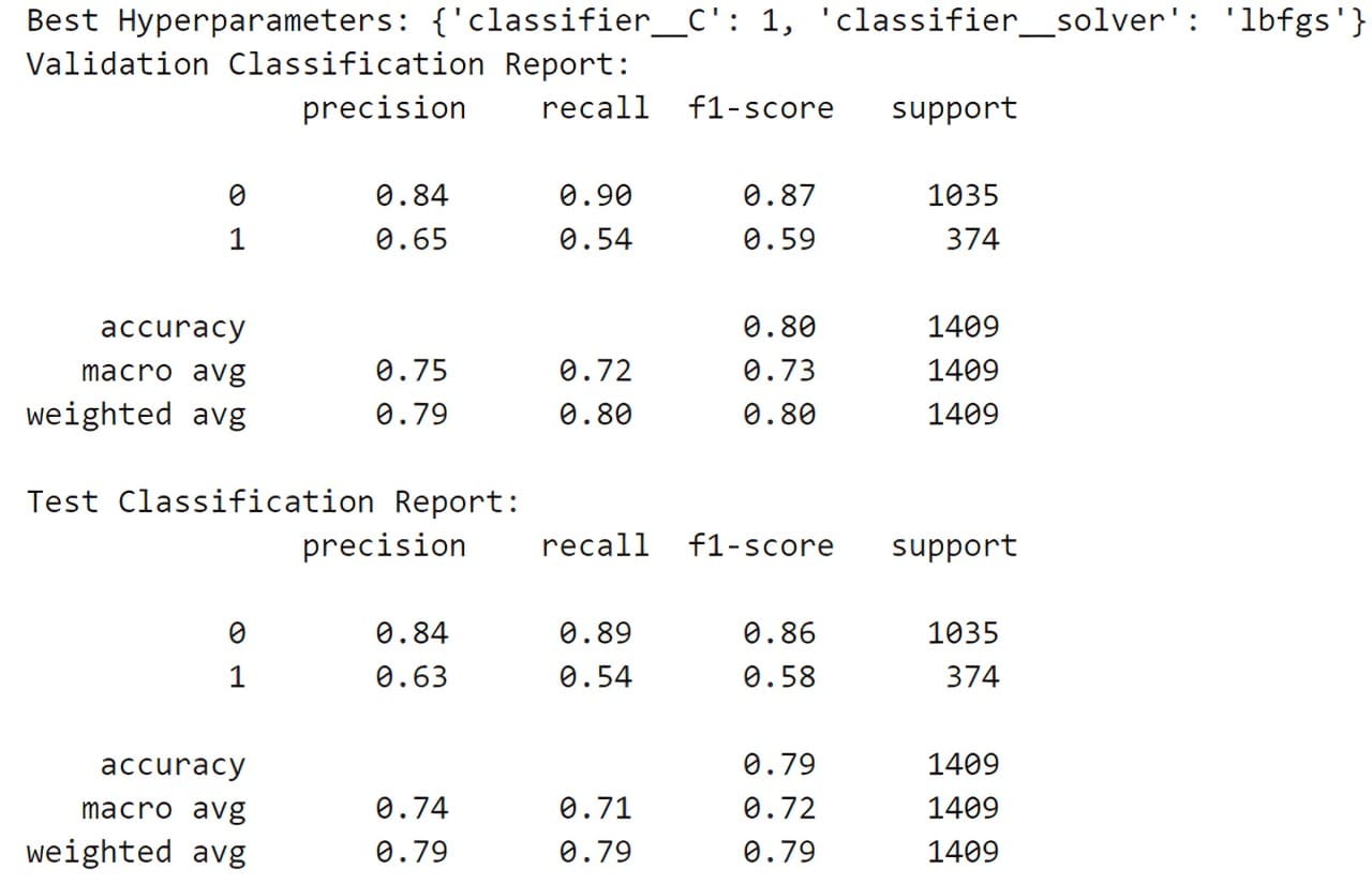
print("Best Hyperparameters:", grid_search.best_params_)

# Evaluate on the validation set
y_val_pred = grid_search.predict(X_val)
print("Validation Classification Report:n", classification_report(y_val, y_val_pred))

# Evaluate on the test set
y_test_pred = grid_search.predict(X_test)
print("Test Classification Report:n", classification_report(y_test, y_test_pred))

The results still do not show the best recall score, but this is expected as they are only the baseline model. Let’s experiment with several models to see if the Recall performance improves. You can always tweak the hyperparameter below.

from sklearn.tree import DecisionTreeClassifier
from sklearn.ensemble import RandomForestClassifier, GradientBoostingClassifier
from sklearn.svm import SVC
from xgboost import XGBClassifier
from lightgbm import LGBMClassifier
from sklearn.metrics import recall_score

# Define the models and their parameter grids
models = {
    'Logistic Regression': {
        'model': LogisticRegression(max_iter=1000),
        'params': {
            'classifier__C': [0.1, 1, 10, 100],
            'classifier__solver': ['lbfgs', 'liblinear']
        }
    },
    'Decision Tree': {
        'model': DecisionTreeClassifier(),
        'params': {
            'classifier__max_depth': [None, 10, 20, 30],
            'classifier__min_samples_split': [2, 10, 20]
        }
    },
    'Random Forest': {
        'model': RandomForestClassifier(),
        'params': {
            'classifier__n_estimators': [100, 200],
            'classifier__max_depth': [None, 10, 20]
        }
    },
    'SVM': {
        'model': SVC(),
        'params': {
            'classifier__C': [0.1, 1, 10, 100],
            'classifier__kernel': ['linear', 'rbf']
        }
    },
    'Gradient Boosting': {
        'model': GradientBoostingClassifier(),
        'params': {
            'classifier__n_estimators': [100, 200],
            'classifier__learning_rate': [0.01, 0.1, 0.2]
        }
    },
    'XGBoost': {
        'model': XGBClassifier(use_label_encoder=False, eval_metric='logloss'),
        'params': {
            'classifier__n_estimators': [100, 200],
            'classifier__learning_rate': [0.01, 0.1, 0.2],
            'classifier__max_depth': [3, 6, 9]
        }
    },
    'LightGBM': {
        'model': LGBMClassifier(),
        'params': {
            'classifier__n_estimators': [100, 200],
            'classifier__learning_rate': [0.01, 0.1, 0.2],
            'classifier__num_leaves': [31, 50, 100]
        }
    }
}

results = []

# Train and evaluate each model
for model_name, model_info in models.items():
    pipeline = Pipeline(steps=[
        ('preprocessor', preprocessor),
        ('classifier', model_info['model'])
    ])
    
    grid_search = GridSearchCV(pipeline, model_info['params'], cv=5, scoring='recall')
    grid_search.fit(X_train, y_train)
    
    # Best model from Grid Search
    best_model = grid_search.best_estimator_
    
    # Evaluate on the validation set
    y_val_pred = best_model.predict(X_val)
    val_recall = recall_score(y_val, y_val_pred, pos_label=1)
    
    # Evaluate on the test set
    y_test_pred = best_model.predict(X_test)
    test_recall = recall_score(y_test, y_test_pred, pos_label=1)
    
    # Save results
    results.append({
        'model': model_name,
        'best_params': grid_search.best_params_,
        'val_recall': val_recall,
        'test_recall': test_recall,
        'classification_report_val': classification_report(y_val, y_val_pred),
        'classification_report_test': classification_report(y_test, y_test_pred)
    })

# Plot the test recall scores
plt.figure(figsize=(10, 6))
model_names = [result['model'] for result in results]
test_recalls = [result['test_recall'] for result in results]
plt.barh(model_names, test_recalls, color='skyblue')
plt.xlabel('Test Recall')
plt.title('Comparison of Test Recall for Different Models')
plt.show()

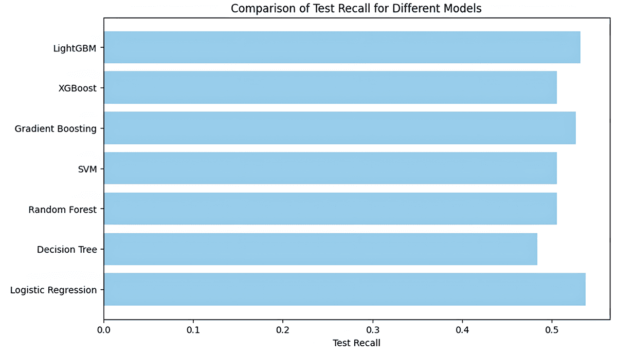
The recall result has not changed much; even the baseline Logistic Regression seems the best. We should return with a better feature selection if we want a better result.

However, let’s move forward with the current Logistic Regression model and try to deploy them.
 

5. Deploying the Model

 
We have built our machine learning model. After having the model, the next step is to deploy it into production. Let’s simulate it using a simple API.

First, let’s develop our model again and save it as a joblib object.

import joblib

best_params = {'classifier__C': 1, 'classifier__solver': 'lbfgs'}
logreg_model = LogisticRegression(C=best_params['classifier__C'], solver=best_params['classifier__solver'], max_iter=1000)

preprocessor = ColumnTransformer(
    transformers=[
        ('num', 'passthrough', num_features),
        ('cat', OneHotEncoder(), cat_features)

pipeline = Pipeline(steps=[
    ('preprocessor', preprocessor),
    ('classifier', logreg_model)
])

pipeline.fit(X_train, y_train)

# Save the model
joblib.dump(pipeline, 'logreg_model.joblib')

Once the model object is ready, we will move into a Python script to create the API. But first, we need to install a few packages used for deployment.

pip install fastapi uvicorn

We would not do it in the notebook but in an IDE such as Visual Studio Code. In your preferred IDE, create a Python script called app.py and put the code below into the script.

from fastapi import FastAPI
from pydantic import BaseModel
import joblib
import numpy as np

# Load the logistic regression model pipeline
model = joblib.load('logreg_model.joblib')

# Define the input data for model
class CustomerData(BaseModel):
    tenure: int
    InternetService: str
    OnlineSecurity: str
    TechSupport: str
    Contract: str
    PaymentMethod: str

# Create FastAPI app
app = FastAPI()

# Define prediction endpoint
@app.post("/predict")
def predict(data: CustomerData):
    # Convert input data to a dictionary and then to a DataFrame
    input_data = {
        'tenure': [data.tenure],
        'InternetService': [data.InternetService],
        'OnlineSecurity': [data.OnlineSecurity],
        'TechSupport': [data.TechSupport],
        'Contract': [data.Contract],
        'PaymentMethod': [data.PaymentMethod]
    }
   
    import pandas as pd
    input_df = pd.DataFrame(input_data)
   
    # Make a prediction
    prediction = model.predict(input_df)
   
    # Return the prediction
    return {"prediction": int(prediction[0])}

if __name__ == "__main__":
    import uvicorn
    uvicorn.run(app, host="0.0.0.0", port=8000)

In your command prompt or terminal, run the following code.

uvicorn app:app --reload

With the code above, we already have an API to accept data and create predictions. Let’s try it out with the following code in the new terminal.

curl -X POST "http://127.0.0.1:8000/predict" -H "Content-Type: application/json" -d "{"tenure": 72, "InternetService": "Fiber optic", "OnlineSecurity": "Yes", "TechSupport": "Yes", "Contract": "Two year", "PaymentMethod": "Credit card (automatic)"}"

Output>>
{"prediction":0}

As you can see, the API result is a dictionary with prediction 0 (Not-Churn). You can tweak the code even further to get the desired result.

Congratulation. You have developed your machine learning model and successfully deployed it in the API.
 

Conclusion

 
We have learned how to develop a machine learning model from the beginning to the deployment. Experiment with other datasets and use cases to get the feeling even better. All the code this article uses will be available on my GitHub repository.
 
 

Cornellius Yudha Wijaya is a data science assistant manager and data writer. While working full-time at Allianz Indonesia, he loves to share Python and data tips via social media and writing media. Cornellius writes on a variety of AI and machine learning topics.

• SEO Powered Content & PR Distribution. Get Amplified Today.
• PlatoData.Network Vertical Generative Ai. Empower Yourself. Access Here.
• PlatoAiStream. Web3 Intelligence. Knowledge Amplified. Access Here.
• PlatoESG. Carbon, CleanTech, Energy, Environment, Solar, Waste Management. Access Here.
• PlatoHealth. Biotech and Clinical Trials Intelligence. Access Here.
• Source: https://www.kdnuggets.com/step-by-step-tutorial-to-building-your-first-machine-learning-model?utm_source=rss&utm_medium=rss&utm_campaign=step-by-step-tutorial-to-building-your-first-machine-learning-model