Image from Bing Image Creator

Exploratory Data Analysis (EDA) is the single most important task to conduct at the beginning of every data science project.

In essence, it involves thoroughly examining and characterizing your data in order to find its underlying characteristics, possible anomalies, and hidden patterns and relationships.

This understanding of your data is what will ultimately guide through the following steps of you machine learning pipeline, from data preprocessing to model building and analysis of results.

The process of EDA fundamentally comprises three main tasks:

• Step 1: Dataset Overview and Descriptive Statistics
• Step 2: Feature Assessment and Visualization, and
• Step 3: Data Quality Evaluation

As you may have guessed, each of these tasks may entail a quite comprehensive amount of analyses, which will easily have you slicing, printing, and plotting your pandas dataframes like a madman.

Unless you pick the right tool for the job.

In this article, we’ll dive into each step of an effective EDA process, and discuss why you should turn ydata-profiling into your one-stop shop to master it.

To demonstrate best practices and investigate insights, we’ll be using the Adult Census Income Dataset, freely available on Kaggle or UCI Repository (License: CC0: Public Domain).

When we first get our hands on an unknown dataset, there is an automatic thought that pops up right away: What am I working with?

We need to have a deep understanding of our data to handle it efficiently in future machine learning tasks

As a rule of thumb, we traditionally start by characterizing the data relatively to the number of observations, number and types of features, overall missing rate, and percentage of duplicate observations.

With some pandas manipulation and the right cheatsheet, we could eventually print out the above information with some short snippets of code:

Dataset Overview: Adult Census Dataset. Number of observations, features, feature types, duplicated rows, and missing values. Snippet by Author.

All in all, the output format is not ideal… If you’re familiar with pandas, you’ll also know the standard modus operandi of starting an EDA process — df.describe():

Adult Dataset: Main statistics presented with df.describe(). Image by Author.

This however, only considers numeric features. We could use a df.describe(include='object') to print out some additional information on categorical features (count, unique, mode, frequency), but a simple check of existing categories would involve something a little more verbose:

Dataset Overview: Adult Census Dataset. Printing the existing categories and respective frequencies for each categorical feature in data. Snippet by Author.

However, we can do this — and guess what, all of the subsequent EDA tasks! — in a single line of code, using ydata-profiling:

Profiling Report of the Adult Census Dataset, using ydata-profiling. Snippet by Author.

The above code generates a complete profiling report of the data, which we can use to further move our EDA process, without the need to write any more code!

We’ll go through the various sections of the report in the following sections. In what concerns the overall characteristics of the data, all the information we were looking for is included in the Overview section:

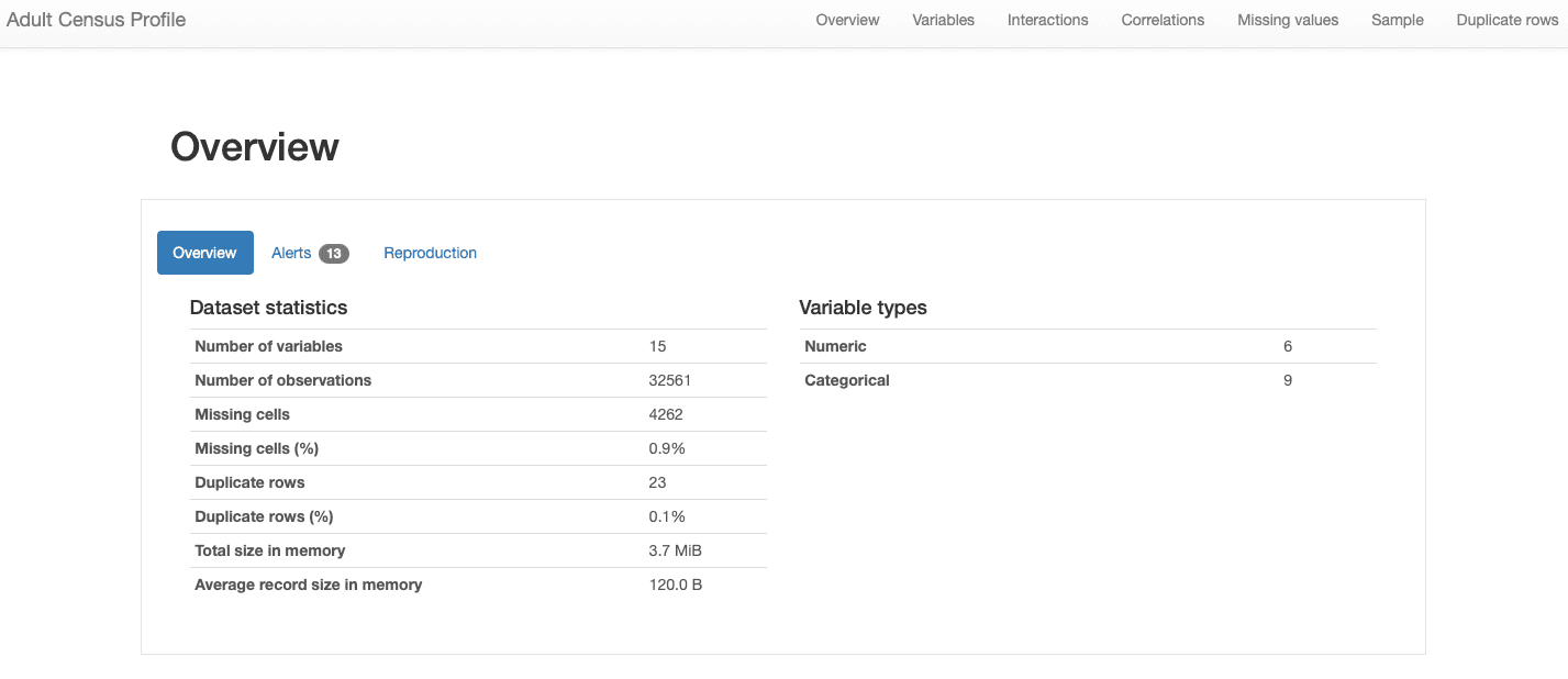
ydata-profiling: Data Profiling Report — Dataset Overview. Image by Author.

We can see that our dataset comprises 15 features and 32561 observations, with 23 duplicate records, and an overall missing rate of 0.9%.

Additionally, the dataset has been correctly identified as a tabular dataset, and rather heterogeneous, presenting both numerical and categorical features. For time-series data, which has time dependency and presents different types of patterns, ydata-profiling would incorporate other statistics and analysis in the report.

We can further inspect the raw data and existing duplicate records to have an overall understanding of the features, before going into more complex analysis:

ydata-profiling: Data Profiling Report — Sample preview. Image by Author.

From the brief sample preview of the data sample, we can see right away that although the dataset has a low percentage of missing data overall, some features might be affected by it more than others. We can also identify a rather considerable number of categories for some features, and 0-valued features (or at least with a significant amount of 0’s).

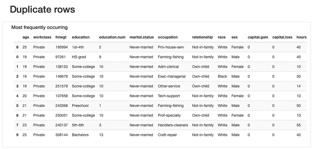
ydata-profiling: Data Profiling Report — Duplicate rows preview. Image by Author.

Regarding the duplicate rows, it would not be strange to find “repeated” observations given that most features represent categories where several people might “fit in” simultaneously.

Yet, perhaps a “data smell” could be that these observations share the same age values (which is plausible) and the exact same fnlwgt which, considering the presented values, seems harder to believe. So further analysis would be required, but we should most likely drop these duplicates later on.

Overall, the data overview might be a simple analysis, but one extremely impactful, as it will help us define the upcoming tasks in our pipeline.

After having a peek at the overall data descriptors, we need to zoom in on our dataset’s features, in order to get some insights on their individual properties — Univariate Analysis — as well their interactions and relationships — Multivariate Analysis.

Both tasks rely heavily on investigating adequate statistics and visualizations, which need to be to tailored to the type of feature at hand (e.g., numeric, categorical), and the behavior we’re looking to dissect (e.g., interactions, correlations).

Let’s take a look at best practices for each task.

Univariate Analysis

Analyzing the individual characteristics of each feature is crucial as it will help us decide on their relevance for the analysis and the type of data preparation they may require to achieve optimal results.

For instance, we may find values that are extremely out of range and may refer to inconsistencies or outliers. We may need to standardize numerical data or perform a one-hot encoding of categorical features, depending on the number of existing categories. Or we may have to perform additional data preparation to handle numeric features that are shifted or skewed, if the machine learning algorithm we intend to use expects a particular distribution (normally Gaussian).

Best practices therefore call for the thorough investigation of individual properties such as descriptive statistics and data distribution.

These will highlight the need for subsequent tasks of outlier removal, standardization, label encoding, data imputation, data augmentation, and other types of preprocessing.

Let’s investigate race and capital.gain in more detail. What can we immediately spot?

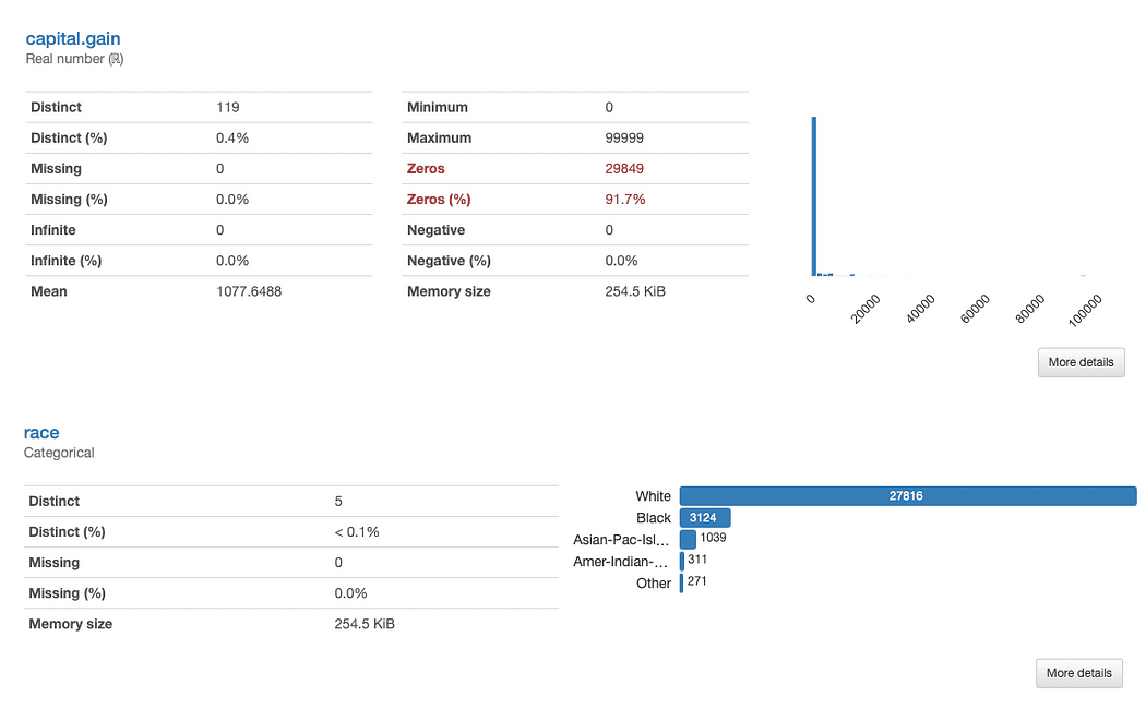
ydata-profiling: Profiling Report (race and capital.gain). Image by Author.

The assessment of capital.gain is straightforward:

Given the data distribution, we might question if the feature adds any value to our analysis, as 91.7% of values are “0”.

Analyzing race is slightly more complex:

There’s a clear underrepresentation of races other than White. This brings two main issues to mind:

• One is the general tendency of machine learning algorithms to overlook less represented concepts, known as the problem of small disjuncts, that leads to reduced learning performance;
• The other is somewhat derivative of this issue: as we’re dealing with a sensitive feature, this “overlooking tendency” may have consequences that directly relate to bias and fairness issues. Something that we definitely don’t want to creep into our models.

Taking this into account, maybe we should consider performing data augmentation conditioned on the underrepresented categories, as well as considering fairness-aware metrics for model evaluation, to check for any discrepancies in performance that relate to race values.

We will further detail on other data characteristics that need to be addressed when we discuss data quality best practices (Step 3). This example just goes to show how much insights we can take just by assessing each individual feature’s properties.

Finally, note how, as previously mentioned, different feature types call for different statistics and visualization strategies:

• Numeric features most often comprise information regarding mean, standard deviation, skewness, kurtosis, and other quantile statistics, and are best represented using histogram plots;
• Categorical features are usually described using the mode, median, and frequency tables, and represented using bar plots for category analysis.

ydata-profiling: Profiling Report. Presented statistics and visualizations are adjusted to each feature type. Screencast by Author.

Such a detailed analysis would be cumbersome to carry out with general pandas manipulation, but fortunately ydata-profiling has all of this functionality built into the ProfileReport for our convenience: no extra lines of code were added to the snippet!

Multivariate Analysis

For Multivariate Analysis, best practices focus mainly on two strategies: analyzing the interactions between features, and analyzing their correlations.

Analyzing Interactions

Interactions let us visually explore how each pair of features behaves, i.e., how the values of one feature relate to the values of the other.

For instance, they may exhibit positive or negative relationships, depending on whether the increase of one’s values is associated with an increase or decrease of the values of the other, respectively.

ydata-profiling: Profiling Report — Interactions. Image by Author.

Taking the interaction between age and hours.per.weekas an example, we can see that the great majority of the working force works a standard of 40 hours. However, there are some “busy bees” that work past that (up until 60 or even 65 hours) between the ages of 30 and 45. People in their 20’s are less likely to overwork, and may have a more light work schedule on some weeks.

Analyzing Correlations

Similarly to interactions, correlations let us analyze the relationship between features. Correlations, however, “put a value” on it, so that it is easier for us to determine the “strength” of that relationship.

This “strength” is measured by correlation coefficients and can be analyzed either numerically (e.g., inspecting a correlation matrix) or with a heatmap, that uses color and shading to visually highlight interesting patterns:

ydata-profiling: Profiling Report — Heatmap and Correlation Matrix. Screencast by Author.

Regarding our dataset, notice how the correlation between education and education.num stands out. In fact, they hold the same information, and education.num is just a binning of the education values.

Other pattern that catches the eye is the the correlation between sex and relationship although again not very informative: looking at the values of both features, we would realize that these features are most likely related because male and female will correspond to husband and wife, respectively.

These type of redundancies may be checked to see whether we may remove some of these features from the analysis (marital.status is also related to relationship and sex; native.country and race for instance, among others).

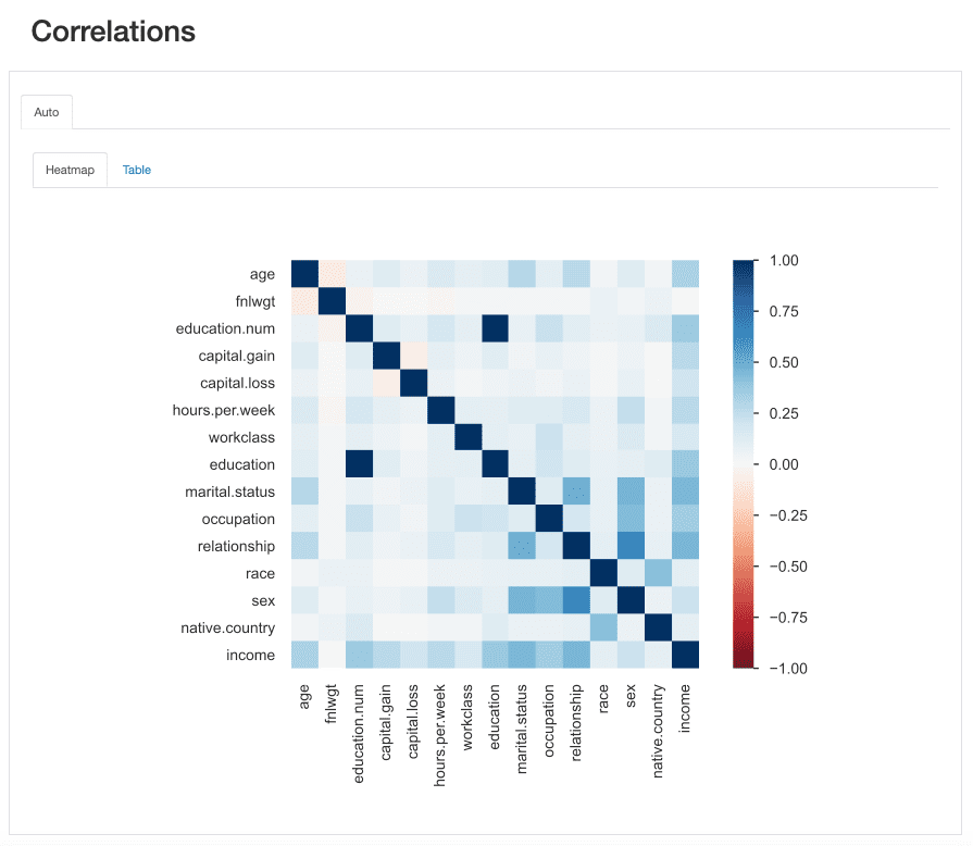
ydata-profiling: Profiling Report — Correlations. Image by Author.

However, there are other correlations that stand out and could be interesting for the purpose of our analysis.

For instance, the correlation betweensex and occupation, or sex and hours.per.week.

Finally, the correlations between income and the remaining features are truly informative, specially in case we’re trying to map out a classification problem. Knowing what are the most correlated features to our target class helps us identify the most discriminative features and well as find possible data leakers that may affect our model.

From the heatmap, seems that marital.status or relationship are amongst the most important predictors, while fnlwgt for instance, does not seem to have a great impact on the outcome.

Similarly to data descriptors and visualizations, interactions and correlations also need to attend to the types of features at hand.

In other words, different combinations will be measured with different correlation coefficients. By default, ydata-profiling runs correlations on auto, which means that:

• Numeric versus Numeric correlations are measured using Spearman’s rank correlation coefficient;
• Categorical versus Categorical correlations are measured using Cramer’s V;
• Numeric versus Categorical correlations also use Cramer’s V, where the numeric feature is first discretized;

And if you want to check other correlation coefficients (e.g., Pearson’s, Kendall’s, Phi) you can easily configure the report’s parameters.

As we navigate towards a data-centric paradigm of AI development, being on top of the possible complicating factors that arise in our data is essential.

With “complicating factors”, we refer to errors that may occurs during the data collection of processing, or data intrinsic characteristics that are simply a reflection of the nature of the data.

These include missing data, imbalanced data, constant values, duplicates, highly correlated or redundant features, noisy data, among others.

Data Quality Issues: Errors and Data Intrinsic Charcateristics. Image by Author.

Finding these data quality issues at the beginning of a project (and monitoring them continuously during development) is critical.

If they are not identified and addressed prior to the model building stage, they can jeopardize the whole ML pipeline and the subsequent analyses and conclusions that may derive from it.

Without an automated process, the ability to identify and address these issues would be left entirely to the personal experience and expertise of the person conducting the EDA analysis, which is obvious not ideal. Plus, what a weight to have on one’s shoulders, especially considering high-dimensional datasets. Incoming nightmare alert!

This is one of the most highly appreciated features of ydata-profiling, the automatic generation of data quality alerts:

ydata-profiling: Profiling Report — Data Quality Alerts. Image by Author.

The profile outputs at least 5 different types of data quality issues, namely duplicates, high correlation, imbalance, missing, and zeros.

Indeed, we had already identified some of these before, as we went through step 2: race is a highly imbalanced feature and capital.gain is predominantly populated by 0’s. We’ve also seen the tight correlation between education and education.num, and relationship and sex.

Analyzing Missing Data Patterns

Among the comprehensive scope of alerts considered, ydata-profiling is especially helpful in analyzing missing data patterns.

Since missing data is a very common problem in real-world domains and may compromise the application of some classifiers altogether or severely bias their predictions, another best practice is to carefully analyze the missing data percentage and behavior that our features may display:

ydata-profiling: Profiling Report — Analyzing Missing Values. Screencast by Author.

From the data alerts section, we already knew that workclass, occupation, and native.country had absent observations. The heatmap further tells us that there is a direct relationship with the missing pattern in occupation and workclass: when there’s a missing value in one feature, the other will also be missing.

Key Insight: Data Profiling goes beyond EDA!

So far, we’ve been discussing the tasks that make up a thorough EDA process and how the assessment of data quality issues and characteristics — a process we can refer to as Data Profiling — is definitely a best practice.

Yet, it is important do clarify that data profiling goes beyond EDA. Whereas we generally define EDA as the exploratory, interactive step before developing any type of data pipeline, data profiling is an iterative process that should occur at every step of data preprocessing and model building.

An efficient EDA lays the foundation of a successful machine learning pipeline.

It’s like running a diagnosis on your data, learning everything you need to know about what it entails — its properties, relationships, issues — so that you can later address them in the best way possible.

It’s also the start of our inspiration phase: it’s from EDA that questions and hypotheses start arising, and analysis are planned to validate or reject them along the way.

Throughout the article, we’ve covered the 3 main fundamental steps that will guide you through an effective EDA, and discussed the impact of having a top-notch tool — ydata-profiling — to point us in the right direction, and save us a tremendous amount of time and mental burden.

I hope this guide will help you master the art of “playing data detective” and as always, feedback, questions, and suggestions are much appreciated. Let me know what other topics would like me to write about, or better yet, come meet me at the Data-Centric AI Community and let’s collaborate!

 
 
Miriam Santos focus on educating the Data Science & Machine Learning Communities on how to move from raw, dirty, “bad” or imperfect data to smart, intelligent, high-quality data, enabling machine learning classifiers to draw accurate and reliable inferences across several industries (Fintech, Healthcare & Pharma, Telecomm, and Retail).

 
Original. Reposted with permission.
 

• SEO Powered Content & PR Distribution. Get Amplified Today.
• EVM Finance. Unified Interface for Decentralized Finance. Access Here.
• Quantum Media Group. IR/PR Amplified. Access Here.
• PlatoAiStream. Web3 Data Intelligence. Knowledge Amplified. Access Here.
• Source: https://www.kdnuggets.com/2023/06/data-scientist-essential-guide-exploratory-data-analysis.html?utm_source=rss&utm_medium=rss&utm_campaign=a-data-scientists-essential-guide-to-exploratory-data-analysis