Image by Author
 

Every machine learning model that you train has a set of parameters or model coefficients. The goal of the machine learning algorithm—formulated as an optimization problem—is to learn the optimal values of these parameters. 

In addition, machine learning models also have a set of hyperparameters. Such as the value of K, the number of neighbors, in the K-Nearest Neighbors algorithm. Or the batch size when training a deep neural network, and more.

These hyperparameters are not learned by the model. But rather specified by the developer. They influence model performance and are tunable. So how do you find the best values for these hyperparameters? This process is called hyperparameter optimization or hyperparameter tuning.

The two most common hyperparameter tuning techniques include:

• Grid search
• Randomized search

In this guide, we’ll learn how these techniques work and their scikit-learn implementation.

Let’s start by training a simple Support Vector Machine (SVM) classifier on the wine dataset. 

First, import the required modules and classes: 

from sklearn import datasets
from sklearn.model_selection import train_test_split
from sklearn.svm import SVC
from sklearn.metrics import accuracy_score

The wine dataset is part of the built-in datasets in scikit-learn. So let’s read in the features and the target labels as shown:

# Load the Wine dataset
wine = datasets.load_wine()
X = wine.data
y = wine.target

The wine dataset is a simple dataset with 13 numeric features and three output class labels. It’s a good candidate dataset to learn your way around multi-class classification  problems. You can run wine.DESCR to get a description of the dataset.

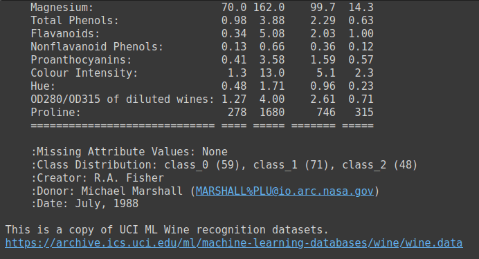
Output of wine.DESCR 
 

Next, split the dataset into train and test sets. Here we’ve used a test_size of 0.2. So 80% of the data goes into the training dataset and 20% to the test dataset.

# Split the dataset into training and testing sets
X_train, X_test, y_train, y_test = train_test_split(X, y, test_size=0.2, random_state=24)

Now instantiate a support vector classifier and fit the model to the training dataset. Then evaluate its performance on the test set.

# Create a baseline SVM classifier
baseline_svm = SVC()
baseline_svm.fit(X_train, y_train)
y_pred = baseline_svm.predict(X_test)

Because it is a simple multi-classification problem, we can look at the model’s accuracy.

# Evaluate the baseline model
accuracy = accuracy_score(y_test, y_pred)
print(f"Baseline SVM Accuracy: {accuracy:.2f}")

We see that the accuracy score of this model with the default values for hyperparameters is about 0.78. 

Output >>>
Baseline SVM Accuracy: 0.78

Here we used a random_state of 24. For a different random state you will get a different training test split, and subsequently different accuracy score.

So we need a better way than a single train-test split to evaluate the model’s performance. Perhaps, train the model on many such splits and consider the average accuracy. While also trying out different combinations of hyperparameters? Yes, that is why we use cross validation in model evaluation and hyperparameter search. We’ll learn more in the following sections.

Next let’s identify the hyperparameters that we cantune for this support vector machine classifier.

In hyperparameter tuning, we aim to find the best combination of hyperparameter values for our SVM classifier. The commonly tuned hyperparameters for the support vector classifier include:

• C: Regularization parameter, controlling the trade-off between maximizing the margin and minimizing classification error.
• kernel: Specifies the type of kernel function to use (e.g., ‘linear,’ ‘rbf,’ ‘poly’).
• gamma: Kernel coefficient for ‘rbf’ and ‘poly’ kernels.

Cross-validation helps assess how well the model generalizes to unseen data and reduces the risk of overfitting to a single train-test split. The commonly used k-fold cross-validation involves splitting the dataset into k equally sized folds. The model is trained k times, with each fold serving as the validation set once and the remaining folds as the training set. So for each fold, we’ll get a cross-validation accuracy.

When we run the grid and randomized searches for finding the best hyperparameters, we’ll choose the hyperparameters based on the best average cross-validation score.

Grid search is a hyperparameter tuning technique that performs an exhaustive search over a specified hyperparameter space to find the combination of hyperparameters that yields the best model performance.

How Grid Search Works

We define the hyperparameter search space as a parameter grid. The parameter grid is a dictionary where you specify each hyperparameter you want to tune with a list of values to explore. 

Grid search then systematically explores every possible combination of hyperparameters from the parameter grid. It fits and evaluates the model for each combination using cross-validation and selects the combination that yields the best performance.

Next, let’s implement grid search in scikit-learn.

First, import the GridSearchCV class from scikit-learn’s model_selection module:

from sklearn.model_selection import GridSearchCV

Let’s define the parameter grid for the SVM classifier:

# Define the hyperparameter grid
param_grid = { 'C': [0.1, 1, 10], 'kernel': ['linear', 'rbf', 'poly'], 'gamma': [0.1, 1, 'scale', 'auto']
}

Grid search then systematically explores every possible combination of hyperparameters from the parameter grid. For this example, it evaluates the model’s performance with:

• C set to 0.1, 1, and 10,
• kernel set to ‘linear’, ‘rbf’, and ‘poly’, and
• gamma set to 0.1, 1, ‘scale’, and ‘auto’.

This results in a total of 3 * 3 * 4 = 36 different combinations to evaluate. Grid search fits and evaluates the model for each combination using cross-validation and selects the combination that yields the best performance.

We then instantiate GridSearchCV to tune the hyperparameters of the baseline_svm:

# Create the GridSearchCV object
grid_search = GridSearchCV(estimator=baseline_svm, param_grid=param_grid, cv=5) # Fit the model with the grid of hyperparameters
grid_search.fit(X_train, y_train)

Note that we’ve used 5-fold cross-validation. 

Finally, we evaluate the performance of the best model—with the optimal hyperparameters found by grid search—on the test data:

# Get the best hyperparameters and model
best_params = grid_search.best_params_
best_model = grid_search.best_estimator_ # Evaluate the best model
y_pred_best = best_model.predict(X_test)
accuracy_best = accuracy_score(y_test, y_pred_best)
print(f"Best SVM Accuracy: {accuracy_best:.2f}")
print(f"Best Hyperparameters: {best_params}")

As seen, the model achieves an accuracy score of 0.94 for the following hyperparameters:

Output >>>
Best SVM Accuracy: 0.94
Best Hyperparameters: {'C': 0.1, 'gamma': 0.1, 'kernel': 'poly'}

Using grid search for hyperparameter tuning has the following advantages:

• Grid search explores all specified combinations, ensuring you don’t miss the best hyperparameters within the defined search space.
• It is a good choice for exploring smaller hyperparameter spaces.

On the flip side, however:

• Grid search can be computationally expensive, especially when dealing with a large number of hyperparameters and their values. It may not be feasible for very complex models or extensive hyperparameter searches.

Now let’s learn about randomized search.

Randomized search is another hyperparameter tuning technique that explores random combinations of hyperparameters within specified distributions or ranges. It’s particularly useful when dealing with a large hyperparameter search space.

How Randomized Search Works 

In randomized search, instead of specifying a grid of values, you can define probability distributions or ranges for each hyperparameter. Which becomes a much larger hyperparameter search space.

Randomized search then randomly samples a fixed number of combinations of hyperparameters from these distributions. This allows randomized search to explore a diverse set of hyperparameter combinations efficiently.

Now let’s tune the parameters of the baseline SVM classifier using randomized search.

We import the RandomizedSearchCV class and define param_dist, a much larger hyperparameter search space:

from sklearn.model_selection import RandomizedSearchCV
from scipy.stats import uniform param_dist = { 'C': uniform(0.1, 10), # Uniform distribution between 0.1 and 10 'kernel': ['linear', 'rbf', 'poly'], 'gamma': ['scale', 'auto'] + list(np.logspace(-3, 3, 50))
}

Similar to grid search, we instantiate the randomized search model to search for the best hyperparameters. Here, we set n_iter to 20; so 20 random hyperparameter combinations will be sampled.

# Create the RandomizedSearchCV object
randomized_search = RandomizedSearchCV(estimator=baseline_svm, param_distributions=param_dist, n_iter=20, cv=5) randomized_search.fit(X_train, y_train)

We then evaluate model’s performance with the best hyper parameters found through randomized search:

# Get the best hyperparameters and model
best_params_rand = randomized_search.best_params_
best_model_rand = randomized_search.best_estimator_ # Evaluate the best model
y_pred_best_rand = best_model_rand.predict(X_test)
accuracy_best_rand = accuracy_score(y_test, y_pred_best_rand)
print(f"Best SVM Accuracy: {accuracy_best_rand:.2f}")
print(f"Best Hyperparameters: {best_params_rand}")

The best accuracy and optimal hyperparameters are:

Output >>>
Best SVM Accuracy: 0.94
Best Hyperparameters: {'C': 9.66495227534876, 'gamma': 6.25055192527397, 'kernel': 'poly'}

The parameters found through randomized search are different from those found through grid search. The model with these hyperparameters also achieves an accuracy score of 0.94.

Let’s sum up the advantages of randomized search:

• Randomized search is efficient when dealing with a large number of hyperparameters or a wide range of values because it doesn’t require an exhaustive search.
• It can handle various parameter types, including continuous and discrete values.

Here are some limitations of randomized search:

• Due to its random nature, it may not always find the best hyperparameters. But it often finds good ones quickly.
• Unlike grid search, it doesn’t guarantee that all possible combinations will be explored.

We learned how to perform hyperparameter tuning with RandomizedSearchCV and GridSearchCV in scikit-learn. We then evaluated our model’s performance with the best hyperparameters. 

In summary, grid search exhaustively searches through all possible combinations in the parameter grid. While randomized search randomly samples hyperparameter combinations.

Both these techniques help you identify the optimal hyperparameters for your machine learning model while reducing the risk of overfitting to a specific train-test split.
 
 

Bala Priya C is a developer and technical writer from India. She likes working at the intersection of math, programming, data science, and content creation. Her areas of interest and expertise include DevOps, data science, and natural language processing. She enjoys reading, writing, coding, and coffee! Currently, she’s working on learning and sharing her knowledge with the developer community by authoring tutorials, how-to guides, opinion pieces, and more.

• SEO Powered Content & PR Distribution. Get Amplified Today.
• PlatoData.Network Vertical Generative Ai. Empower Yourself. Access Here.
• PlatoAiStream. Web3 Intelligence. Knowledge Amplified. Access Here.
• PlatoESG. Carbon, CleanTech, Energy, Environment, Solar, Waste Management. Access Here.
• PlatoHealth. Biotech and Clinical Trials Intelligence. Access Here.
• Source: https://www.kdnuggets.com/hyperparameter-tuning-gridsearchcv-and-randomizedsearchcv-explained?utm_source=rss&utm_medium=rss&utm_campaign=hyperparameter-tuning-gridsearchcv-and-randomizedsearchcv-explained