Introduction

Retrieval Augmented-Generation (RAG) has taken the world by Storm ever since its inception. RAG is what is necessary for the Large Language Models (LLMs) to provide or generate accurate and factual answers. We solve the factuality of LLMs by RAG, where we try to give the LLM a context that is contextually similar to the user query so that the LLM will work with this context and generate a factually correct response. We do this by representing our data and user query in the form of vector embeddings and performing a cosine similarity. But the problem is, that all the traditional approaches represent the data in a single embedding, which may not be ideal for good retrieval systems. In this guide, we will look into ColBERT which performs retrieval with better accuracy than traditional bi-encoder models.

Learning Objectives

• Understand how retrieval in RAG works on a high level.
• Understand single embedding limitations in retrieval.
• Improve retrieval context with ColBERT’s token embeddings.
• Learn how ColBERT’s late interaction improves retrieval.
• Get to know how to work with ColBERT for accurate retrieval.

This article was published as a part of the Data Science Blogathon.

What is RAG?

LLMs, although capable of generating text that is both meaningful and grammatically correct, these LLMs suffer from a problem called hallucination. Hallucination in LLMs is the concept where the LLMs confidently generate wrong answers, that is they make up wrong answers in a way that makes us believe that it is true. This has been a major problem since the introduction of the LLMs. These hallucinations lead to incorrect and factually wrong answers. Hence Retrieval Augmented Generation was introduced.

In RAG, we take a list of documents/chunks of documents and encode these textual documents into a numerical representation called vector embeddings, where a single vector embedding represents a single chunk of document and stores them in a database called vector store. The models required for encoding these chunks into embeddings are called encoding models or bi-encoders. These encoders are trained on a large corpus of data, thus making them powerful enough to encode the chunks of documents in a single vector embedding representation.

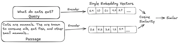
Now when a user asks a query to the LLM, then we give this query to the same encoder to produce a single vector embedding. This embedding is then used to calculate the similarity score with various other vector embeddings of the document chunks to get the most relevant chunk of the document. The most relevant chunk or a list of the most relevant chunks along with the user query are given to the LLM. The LLM then receives this extra contextual information and then generates an answer that is aligned with the context received from the user query. This makes sure that the generated content by the LLM is factual and something that can be traced back if necessary.

The Problem with Traditional Bi-Encoders

The problem with traditional Encoder models like the all-miniLM, OpenAI embedding model, and other encoder models is that they compress the entire text into a single vector embedding representation. These single vector embedding representations are useful because they help in the efficient and quick retrieval of similar documents. However, the problem lies in the contextuality between the query and the document. The single vector embedding may not be sufficient to store the contextual information of a document chunk, thus creating an information bottleneck.

Imagine that 500 words are being compressed to a single vector of size 782. It may not be sufficient to represent such a chunk with a single vector embedding, thus giving subpar results in retrieval in most of the cases. The single vector representation may also fail in cases of complex queries or documents. One such solution would be to represent the document chunk or a query as a list of embedding vectors instead of a single embedding vector, this is where ColBERT comes in.

What is ColBERT?

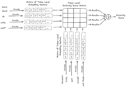
ColBERT (Contextual Late Interactions BERT) is a bi-encoder that represents text in a multi-vector embedding representation. It takes in a Query or a chunk of a Document / a small Document and creates vector embeddings at the token level. That is each token gets its own vector embedding, and the query/document is encoded to a list of token-level vector embeddings. The token level embeddings are generated from a pre-trained BERT model hence the name BERT.

These are then stored in the vector database. Now, when a query comes in, a list of token-level embeddings is created for it and then a matrix multiplication is performed between the user query and each document, thus resulting in a matrix containing similarity scores. The overall similarity is achieved by taking the sum of maximum similarity across the document tokens for each query token. The formula for this can be seen in the below pic:

Here in the above equation, we see that we do a dot product between the Query Tokens Matrix (containing N token level vector embeddings)and the Transpose of Document Tokens Matrix (containing M token level vector embeddings), and then we take the maximum similarity cross the document tokens for each query token. Then we take the sum of all these maximum similarities, which gives us the final similarity score between the document and the query. The reason why this produces effective and accurate retrieval is, that here we are having a token-level interaction, which gives room for more contextual understanding between the query and document.

Why the Name ColBERT?

As we are computing the list of embedding vectors before itself and only performing this MaxSim (maximum similarity) operation during the model inference, thus calling it a late interaction step, and as we are getting more contextual information through token level interactions, it’s called contextual late interactions. Thus the name Contextual Late Interactions BERT or ColBERT. These computations can be performed in parallel, hence they can be computed efficiently. Finally, one concern is the space, that is, it requires a lot of space to store this list of token-level vector embeddings. This issue was solved in the ColBERTv2, where the embeddings are compressed through the technique called residual compression, thus optimizing the space utilized.

Hands-On ColBERT with Example

In this section, we will get hands-on with the ColBERT and even check how it performs against a regular embedding model.

Step 1: Download Libraries

We will start by downloading the following library:

!pip install ragatouille langchain langchain_openai chromadb einops sentence-transformers tiktoken

• RAGatouille: This library lets us work with the state of the art (SOTA) retrieval methods like ColBERT in an easy-to-use way. It provides options to create indexes over the datasets, query on them, and even allow us to train a ColBERT model on our data.
• LangChain: This library will let us work with the open-source embedding models so that we can test how well the other embedding models work when compared to the ColBERT.
• langchain_openai: Installs the LangChain dependencies for OpenAI. We will even work with the OpenAI Embedding model to check its performance against the ColBERT.
• ChromaDB: This library will let us create a vector store in our environment so that we can save the embeddings that we have created on our data and later perform a semantic search between the query and the stored embeddings.
• einops: This library is needed for efficient tensor matrix multiplications.
• sentence-transformers and the tiktoken library are needed for the open-source embedding models to work properly.

Step 2: Download Pre-trained Model

In the next step, we will download the pre-trained ColBERT model. For this, the code will be

from ragatouille import RAGPretrainedModel

RAG = RAGPretrainedModel.from_pretrained("colbert-ir/colbertv2.0")

• We first import the RAGPretrainedModel class from the RAGatouille library.
• Then we call the .from_pretrained() and give the model name i.e. “colbert-ir/colbertv2.0”.

Running the code above will instantiate a ColBERT RAG model. Now let’s download a Wikipedia page and perform retrieval from it. For this, the code will be:

from ragatouille.utils import get_wikipedia_page

document = get_wikipedia_page("Elon_Musk")
print("Word Count:",len(document))
print(document[:1000])

The RAGatouille comes with a handy function called get_wikipedia_page which takes in a string and gets the corresponding Wikipedia page. Here we download the Wikipedia content on Elon Musk and store it in the variable document. Let’s print the number of words present in the document and the first few lines of the document.

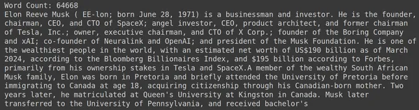
Here we can see the output in the pic. We can see that there are a total of 64,668 words on the Wikipedia page of Elon Musk.

Step 3: Indexing

Now we will create an index on this document.

RAG.index(
   # List of Documents
   collection=[document],
   # List of IDs for the above Documents
   document_ids=['elon_musk'],
   # List of Dictionaries for the metadata for the above Documents
   document_metadatas=[{"entity": "person", "source": "wikipedia"}],
   # Name of the index
   index_name="Elon2",
   # Chunk Size of the Document Chunks
   max_document_length=256,
   # Wether to Split Document or Not
   split_documents=True
   )

Here we call the .index() of the RAG to index our document. To this, we pass the following:

• collection: This is a list of documents that we want to index. Here we have only one document, hence a list of a single document.
• document_ids: Each document expects a unique document ID. Here we pass it the name elon_musk because the document is about Elon Musk.
• document_metadatas: Each document has its metadata to it. This again is a list of dictionaries, where each dictionary contains a key-value pair metadata for a particular document.
• index_name: The name of the index that we are creating. Let’s name it Elon2.
• max_document_size: This is similar to the chunk size. We specify how much should each document chunk be. Here we are giving it a value of 256. If we do not specify any value, 256 will be taken as the default chunk size.
• split_documents: It is a boolean value, where True indicates that we want to split our document according to the given chunk size, and False indicates that we want to store the entire document as a single chunk.

Running the code above will chunk our document in sizes of 256 per chunk, then embed them through the ColBERT model, which will produce a list of token-level vector embeddings for each chunk and finally store them in an index. This step will take a bit of time to run and can be accelerated if having a GPU. Finally, it creates a directory where our index is stored. Here the directory will be “.ragatouille/colbert/indexes/Elon2”

Step 4: General Query

Now, we will begin the search. For this, the code will be

results = RAG.search(query="What companies did Elon Musk find?", k=3, index_name='Elon2')
for i, doc, in enumerate(results):
   print(f"---------------------------------- doc-{i} ------------------------------------")
   print(doc["content"])

• Here, first, we call the .search() method of the RAG object
• To this, we give the variables that include the query name, k (number of documents to retrieve), and the index name to search
• Here we provide the query “What companies did Elon Musk find?”. The result obtained will be in a list of dictionary format, which contains the keys like content, score, rank, document_id, passage_id, and document_metadata
• Hence we work with the code below to print the retrieved documents in a neat way
• Here we go through the list of dictionaries and print the content of the documents

Running the code will produce the following results:

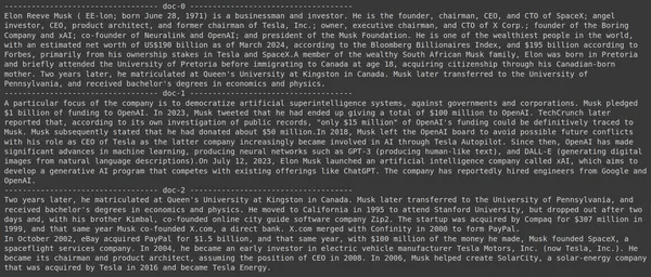
In the pic, we can see that the first and last document entirely covers the different companies founded by Elon Musk. The ColBERT was able to correctly retrieve the relevant chunks needed to answer the query.

Step 5: Specific Query

Now let’s go a step further and ask it a specific question.

results = RAG.search(query="How much Tesla stocks did Elon sold in 
Decemeber 2022?", k=3, index_name='Elon2')


for i, doc, in enumerate(results):
   print(f"---------------
   ------------------- doc-{i} ------------------------------------")
   print(doc["content"])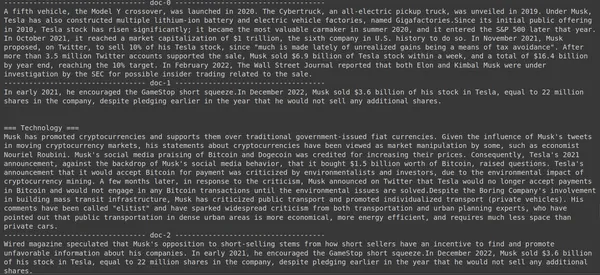

Here in the above code, we are asking a very specific question about how many stocks worth of Tesla Elon sold in the month of December 2022. We can see the output here. The doc-1 contains the answer to the question. Elon has sold $3.6 billion worth of his stock in Tesla. Again, ColBERT was able to successfully retrieve the relevant chunk for the given query.

Step 6: Testing Other Models

Let’s now try the same question with the other embedding models both open-source and closed here:

from langchain_community.embeddings import HuggingFaceEmbeddings
from transformers import AutoModel

model = AutoModel.from_pretrained('jinaai/jina-embeddings-v2-base-en', trust_remote_code=True)

model_name = "jinaai/jina-embeddings-v2-base-en"
model_kwargs = {'device': 'cpu'}

embeddings = HuggingFaceEmbeddings(
   model_name=model_name,
   model_kwargs=model_kwargs,
)

• We start off by downloading the model first through the AutoModel class from the Transformers library.
• Then we store the model_name and the model_kwargs in their respective variables.
• Now to work with this model in LangChain, we import the HuggingFaceEmbeddings from the LangChain and give it the model name and the model_kwargs.

Running this code will download and load the Jina embedding model so that we can work with it

Step 7: Create Embeddings

Now, we need to start splitting our document and then create embeddings out of it and store them in the Chroma vector store. For this, we work with the following code:

from langchain_community.vectorstores import Chroma
from langchain_text_splitters import RecursiveCharacterTextSplitter

text_splitter = RecursiveCharacterTextSplitter.from_tiktoken_encoder(
    chunk_size=256, 
    chunk_overlap=0)
splits = text_splitter.split_text(document)
vectorstore = Chroma.from_texts(texts=splits,
                                embedding=embeddings,
                                collection_name="elon")
retriever = vectorstore.as_retriever(search_kwargs = {'k':3})

• We start by importing the Chroma and the RecursiveCharacterTextSplitter from the LangChain library
• Then we instantiate a text_splitter by calling the .from_tiktoken_encoder of the RecursiveCharacterTextSplitter and passing it the chunk_size and chunk_overlap
• Here we will use the same chunk_size that we have provided to the ColBERT
• Then we call the .split_text() method of this text_splitter and give it the document containing Wikipedia information about Elon Musk. It then splits the document based on the given chunk size and finally, the list of Document Chunks is stored in the variable splits
• Finally, we call the .from_texts() function of the Chroma class to create a vector store. To this function, we give the splits, the embedding model, and the collection_name
• Now, we create a retriever out of it by calling the .as_retriever() function of the vector store object. We give 3 for the k value

Running this code will take our document, split it into smaller documents of size 256 per chunk, and then embed these smaller chunks with the Jina embedding model and store these embedding vectors in the chroma vector store.

Step 8: Creating a Retriever

Finally, we create a retriever from it. Now we will perform a vector search and check the results.

docs = retriever.get_relevant_documents("What companies did Elon Musk find?",)

for i, doc in enumerate(docs):
 print(f"---------------------------------- doc-{i} ------------------------------------")
 print(doc.page_content)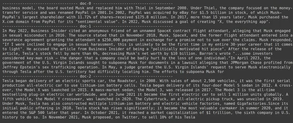

• We call the .get_relevent_documents() function of the retriever object and give it the same query.
• Then we neatly print the top 3 retrieved documents.
• In the pic, we can see that the Jina Embedder despite being a popular embedding model, the retrieval for our query is poor. It was not successful in getting the correct document chunks.

We can clearly spot the difference between the Jina, the embedding model that represents each chunk as a single vector embedding, and the ColBERT model which represents each chunk as a list of token-level embedding vectors. The ColBERT clearly outperforms in this case.

Step 9: Testing OpenAI’s Embedding Model

Now let’s try using a closed-source embedding model like the OpenAI Embedding model.

import os

os.environ["OPENAI_API_KEY"] = "Your API Key"

from langchain_openai import OpenAIEmbeddings

embeddings = OpenAIEmbeddings()

text_splitter = RecursiveCharacterTextSplitter.from_tiktoken_encoder(
              model_name = "gpt-4",
              chunk_size = 256,
              chunk_overlap  = 0,
              )

splits = text_splitter.split_text(document)
vectorstore = Chroma.from_texts(texts=splits,
                                embedding=embeddings,
                                collection_name="elon_collection")

retriever = vectorstore.as_retriever(search_kwargs = {'k':3})

Here the code is very similar to the one that we have just written

• The only difference is, we pass in the OpenAI API key to set the environment variable.
• We then create an instance of the OpenAI Embedding model by importing it from the LangChain.
• And while creating the collection name, we give a different collection name, so that the embeddings from the OpenAI Embedding model are stored in a different collection.

Running this code will again take our documents, chunk them into smaller documents of size 256, and then embed them into single vector embedding representation with the OpenAI embedding model and finally store these embeddings in the Chroma Vector Store. Now let’s try to retrieve the relevant documents to the other question.

docs = retriever.get_relevant_documents("How much Tesla stocks did Elon sold in Decemeber 2022?",)

for i, doc in enumerate(docs):
  print(f"---------------------------------- doc-{i} ------------------------------------")
  print(doc.page_content)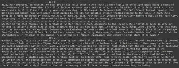

• We see that the answer we are expecting is not found within the retrieved chunks.
• The chunk one contains information about Tesla stocks in 2022 but does not talk about Elon selling them.
• The same can be seen with the remaining two document chunks, where the information they contain is about Tesla and its stock but this is not the information we are expecting.
• The above-retrieved chunks will not provide the context for the LLM to answer the query that we have provided.

Even here we can see a clear difference between the single-vector embedding representation vs the multi-vector embedding representation. The multi-embedding representations clearly capture the complex queries which results in more accurate retrievals.

Conclusion

In conclusion, ColBERT demonstrates a significant advancement in retrieval performance over traditional bi-encoder models by representing text as multi-vector embeddings at the token level. This approach allows for more nuanced contextual understanding between queries and documents, leading to more accurate retrieval results and mitigating the issue of hallucinations commonly observed in LLMs.

Key Takeaways

• RAG addresses the problem of hallucinations in LLMs by providing contextual information for factual answer generation.
• Traditional bi-encoders suffer from an information bottleneck due to compressing entire texts into single vector embeddings, resulting in subpar retrieval accuracy.
• ColBERT, with its token-level embedding representation, facilitates better contextual understanding between queries and documents, leading to improved retrieval performance.
• The late interaction step in ColBERT, combined with token-level interactions, enhances retrieval accuracy by considering contextual nuances.
• ColBERTv2 optimizes storage space through residual compression while maintaining retrieval effectiveness.
• Hands-on experiments demonstrate ColBERT’s superiority in retrieval performance compared to traditional and open-source embedding models like Jina and OpenAI Embedding.

Frequently Asked Questions

The media shown in this article is not owned by Analytics Vidhya and is used at the Author’s discretion.

• SEO Powered Content & PR Distribution. Get Amplified Today.
• PlatoData.Network Vertical Generative Ai. Empower Yourself. Access Here.
• PlatoAiStream. Web3 Intelligence. Knowledge Amplified. Access Here.
• PlatoESG. Carbon, CleanTech, Energy, Environment, Solar, Waste Management. Access Here.
• PlatoHealth. Biotech and Clinical Trials Intelligence. Access Here.
• Source: https://www.analyticsvidhya.com/blog/2024/04/colbert-improve-retrieval-performance-with-token-level-vector-embeddings/