This is a guest post co-authored by Shravan Kumar and Avirat S from Gramener.

Gramener, a Straive company, contributes to sustainable development by focusing on agriculture, forestry, water management, and renewable energy. By providing authorities with the tools and insights they need to make informed decisions about environmental and social impact, Gramener is playing a vital role in building a more sustainable future.

Urban heat islands (UHIs) are areas within cities that experience significantly higher temperatures than their surrounding rural areas. UHIs are a growing concern because they can lead to various environmental and health issues. To address this challenge, Gramener has developed a solution that uses spatial data and advanced modeling techniques to understand and mitigate the following UHI effects:

• Temperature discrepancy – UHIs can cause urban areas to be hotter than their surrounding rural regions.
• Health impact – Higher temperatures in UHIs contribute to a 10-20% increase in heat-related illnesses and fatalities.
• Energy consumption – UHIs amplify air conditioning demands, resulting in an up to 20% surge in energy consumption.
• Air quality – UHIs worsen air quality, leading to elevated levels of smog and particulate matter, which can increase respiratory problems.
• Economic impact – UHIs can result in billions of dollars in additional energy costs, infrastructure damage, and healthcare expenditures.

Gramener’s GeoBox solution empowers users to effortlessly tap into and analyze public geospatial data through its powerful API, enabling seamless integration into existing workflows. This streamlines exploration and saves valuable time and resources, allowing communities to quickly identify UHI hotspots. GeoBox then transforms raw data into actionable insights presented in user-friendly formats like raster, GeoJSON, and Excel, ensuring clear understanding and immediate implementation of UHI mitigation strategies. This empowers communities to make informed decisions and implement sustainable urban development initiatives, ultimately supporting citizens through improved air quality, reduced energy consumption, and a cooler, healthier environment.

This post demonstrates how Gramener’s GeoBox solution uses Amazon SageMaker geospatial capabilities to perform earth observation analysis and unlock UHI insights from satellite imagery. SageMaker geospatial capabilities make it straightforward for data scientists and machine learning (ML) engineers to build, train, and deploy models using geospatial data. SageMaker geospatial capabilities allow you to efficiently transform and enrich large-scale geospatial datasets, and accelerate product development and time to insight with pre-trained ML models.

Solution overview

Geobox aims to analyze and predict the UHI effect by harnessing spatial characteristics. It helps in understanding how proposed infrastructure and land use changes can impact UHI patterns and identifies the key factors influencing UHI. This analytical model provides accurate estimates of land surface temperature (LST) at a granular level, allowing Gramener to quantify changes in the UHI effect based on parameters (names of indexes and data used).

Geobox enables city departments to do the following:

• Improved climate adaptation planning – Informed decisions reduce the impact of extreme heat events.
• Support for green space expansion – More green spaces enhance air quality and quality of life.
• Enhanced interdepartmental collaboration – Coordinated efforts improve public safety.
• Strategic emergency preparedness – Targeted planning reduces the potential for emergencies.
• Health services collaboration – Cooperation leads to more effective health interventions.

Solution workflow

In this section, we discuss how the different components work together, from data acquisition to spatial modeling and forecasting, serving as the core of the UHI solution. The solution follows a structured workflow, with a primary focus on addressing UHIs in a city of Canada.

Phase 1: Data pipeline

The Landsat 8 satellite captures detailed imagery of the area of interest every 15 days at 11:30 AM, providing a comprehensive view of the city’s landscape and environment. A grid system is established with a 48-meter grid size using Mapbox’s Supermercado Python library at zoom level 19, enabling precise spatial analysis.

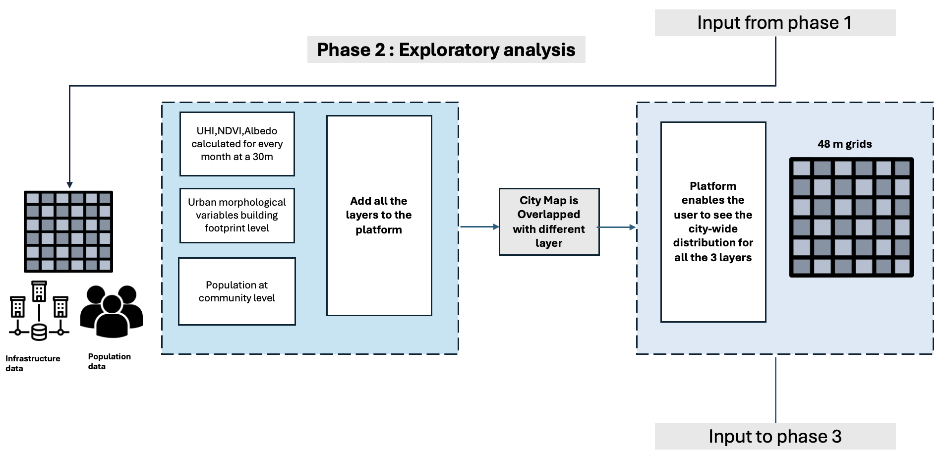
Phase 2: Exploratory analysis

Integrating infrastructure and population data layers, Geobox empowers users to visualize the city’s variable distribution and derive urban morphological insights, enabling a comprehensive analysis of the city’s structure and development.

Also, Landsat imagery from phase 1 is used to derive insights like the Normalized Difference Vegetation Index (NDVI) and Normalized Difference Built-up Index (NDBI), with data meticulously scaled to the 48-meter grid for consistency and accuracy.

The following variables are used:

• Land surface temperature
• Building site coverage
• NDVI
• Building block coverage
• NDBI
• Building area
• Albedo
• Building count
• Modified Normalized Difference Water Index (MNDWI)
• Building height
• Number of floors and floor area
• Floor area ratio

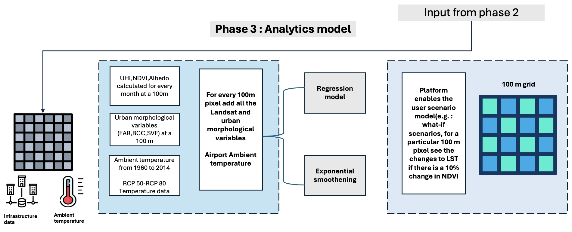
Phase 3: Analytics model

This phase comprises three modules, employing ML models on data to gain insights into LST and its relationship with other influential factors:

• Module 1: Zonal statistics and aggregation – Zonal statistics play a vital role in computing statistics using values from the value raster. It involves extracting statistical data for each zone based on the zone raster. Aggregation is performed at a 100-meter resolution, allowing for a comprehensive analysis of the data.
• Module 2: Spatial modeling – Gramener evaluated three regression models (linear, spatial, and spatial fixed effects) to unravel the correlation between Land Surface Temperature (LST) and other variables. Among these models, the spatial fixed effect model yielded the highest mean R-squared value, particularly for the timeframe spanning 2014 to 2020.
• Module 3: Variables forecasting – To forecast variables in the short term, Gramener employed exponential smoothing techniques. These forecasts aided in understanding future LST values and their trends. Additionally, they delved into long-term scale analysis by using Representative Concentration Pathway (RCP8.5) data to predict LST values over extended periods.

Data acquisition and preprocessing

To implement the modules, Gramener used the SageMaker geospatial notebook within Amazon SageMaker Studio. The geospatial notebook kernel is pre-installed with commonly used geospatial libraries, enabling direct visualization and processing of geospatial data within the Python notebook environment.

Gramener employed various datasets to predict LST trends, including building assessment and temperature data, as well as satellite imagery. The key to the UHI solution was using data from the Landsat 8 satellite. This Earth-imaging satellite, a joint venture of USGS and NASA, served as a fundamental component in the project.

With the SearchRasterDataCollection API, SageMaker provides a purpose-built functionality to facilitate the retrieval of satellite imagery. Gramener used this API to retrieve Landsat 8 satellite data for the UHI solution.

The SearchRasterDataCollection API uses the following input parameters:

• Arn – The Amazon Resource Name (ARN) of the raster data collection used in the query
• AreaOfInterest – A GeoJSON polygon representing the area of interest
• TimeRangeFilter – The time range of interest, denoted as {StartTime: <string>, EndTime: <string>}
• PropertyFilters – Supplementary property filters, such as specifications for maximum acceptable cloud cover, can also be incorporated

The following example demonstrates how Landsat 8 data can be queried via the API:

search_params = {
    "Arn": "arn:aws:sagemaker-geospatial:us-west-2:378778860802:raster-data-collection/public/gmqa64dcu2g9ayx1", # NASA/USGS Landsat
    "RasterDataCollectionQuery": {
        "AreaOfInterest": {
            "AreaOfInterestGeometry": {
                "PolygonGeometry": {
                    "Coordinates": coordinates
                }
            }
        },
        "TimeRangeFilter": {
            "StartTime": "2014-01-01T00:00:00Z",
            "EndTime": "2020-12-31T23:59:59Z",
        },
        "PropertyFilters": {
            "Properties": [{"Property": {"EoCloudCover": {"LowerBound": 0, "UpperBound": 20.0}}}],
            "LogicalOperator": "AND",
        }
    },
}

response = geospatial_client.search_raster_data_collection(**search_params)

To process large-scale satellite data, Gramener used Amazon SageMaker Processing with the geospatial container. SageMaker Processing enables the flexible scaling of compute clusters to accommodate tasks of varying sizes, from processing a single city block to managing planetary-scale workloads. Traditionally, manually creating and managing a compute cluster for such tasks was both costly and time-consuming, particularly due to the complexities involved in standardizing an environment suitable for geospatial data handling.

Now, with the specialized geospatial container in SageMaker, managing and running clusters for geospatial processing has become more straightforward. This process requires minimal coding effort: you simply define the workload, specify the location of the geospatial data in Amazon Simple Storage Service (Amazon S3), and select the appropriate geospatial container. SageMaker Processing then automatically provisions the necessary cluster resources, facilitating the efficient run of geospatial tasks on scales that range from city level to continent level.

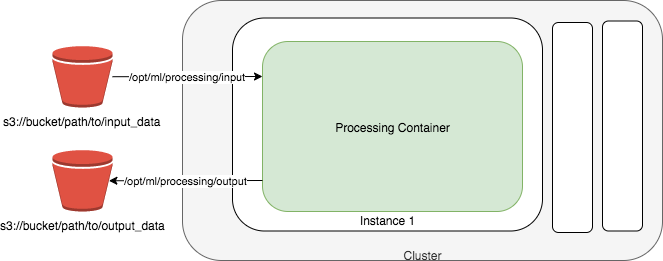
SageMaker fully manages the underlying infrastructure required for the processing job. It allocates cluster resources for the duration of the job and removes them upon job completion. Finally, the results of the processing job are saved in the designated S3 bucket.

A SageMaker Processing job using the geospatial image can be configured as follows from within the geospatial notebook:

from sagemaker import get_execution_role
from sagemaker.sklearn.processing import ScriptProcessor
from sagemaker.processing import ProcessingInput, ProcessingOutput

execution_role_arn = get_execution_role()

geospatial_image_uri = '081189585635.dkr.ecr.us-west-2.amazonaws.com/sagemaker-geospatial-v1-0:latest'
processor = ScriptProcessor(
    command=['python3'],
    image_uri=geospatial_image_uri,
    role=execution_role_arn,
    instance_count=20,
    instance_type='ml.m5.xlarge',
    base_job_name='geospatial-processing-spectral-indices'
)

The instance_count parameter defines how many instances the processing job should use, and the instance_type defines what type of instance should be used.

The following example shows how a Python script is run on the processing job cluster. When the run command is invoked, the cluster starts up and automatically provisions the necessary cluster resources:

processor.run(
    code='calculate_variables.py',
    inputs=[
        ProcessingInput(
            source=s3_manifest_url,
            destination='/opt/ml/processing/input_data/',
            s3_data_type="ManifestFile",
            s3_data_distribution_type="ShardedByS3Key"
        ),
    ],
    outputs=[
        ProcessingOutput(
            source='/opt/ml/processing/output_data/',
            destination=s3_output_prefix_url
        )
    ]
)

Spatial modeling and LST predictions

In the processing job, a range of variables, including top-of-atmosphere spectral radiance, brightness temperature, and reflectance from Landsat 8, are computed. Additionally, morphological variables such as floor area ratio (FAR), building site coverage, building block coverage, and Shannon’s Entropy Value are calculated.

The following code demonstrates how this band arithmetic can be performed:

def calculate_ndvi(nir08, red): 
    return (nir08 - red) / (nir08 + red) 
 
def calculate_ndbi(swir16, nir08): 
    return (swir16 - nir08) / (swir16 + nir08) 
 
def calculate_st(bt): 
    return ((bt * 0.00341802) + 149.0) - 273 
 
def indices_calc(data): 
    with concurrent.futures.ThreadPoolExecutor() as executor: 
        ndvi_future = executor.submit(calculate_ndvi, data.sel(band="SR_B5"), data.sel(band="SR_B4")) 
        ndbi_future = executor.submit(calculate_ndbi, data.sel(band="SR_B6"), data.sel(band="SR_B5")) 
        st_future = executor.submit(calculate_st, data.sel(band="ST_B10")) 
 
        ndvi = ndvi_future.result() 
        ndbi = ndbi_future.result() 
        st = st_future.result() 
 
    ndvi.attrs = data.attrs 
    ndbi.attrs = data.attrs 
    st.attrs = data.attrs 
 
    return ndvi, ndbi, st 

After the variables have been calculated, zonal statistics are performed to aggregate data by grid. This involves calculating statistics based on the values of interest within each zone. For these computations a grid size of approximately 100 meters has been used.

def process_iteration(st, ndvi, ndmi, date, city_name): 
    datacube['st'] = (st.dims, st.values) 
    datacube['ndvi'] = (ndvi.dims, ndvi.values) 
    datacube['ndmi'] = (ndmi.dims, ndmi.values) 
    df = datacube.groupby("id").mean().to_dataframe().reset_index() 
    merged_grid = hexgrid_utm.join(df, on='id', how='left', lsuffix='_')[['id', 'hex_id', 'geometry', 'st', 'ndvi', 'ndmi']] 
    merged_grid.to_file(f"{DATA}/{city_name}/{city_name}_outputs_{date}.geojson", driver='GeoJSON') 
    print("Working on:", date) 
 
def iterative_op(city_json, st, ndvi, ndmi, city_name): 
    with concurrent.futures.ThreadPoolExecutor() as executor: 
        futures = [ 
            executor.submit(process_iteration, st[i], ndvi[i], ndmi[i], date, city_name) 
            for i, _ in enumerate(city_json.time) 
            for date in city_json.date 
        ] 
        for future in concurrent.futures.as_completed(futures): 
            future.result() 
 
    print('Process completed') 

After aggregating the data, spatial modeling is performed. Gramener used spatial regression methods, such as linear regression and spatial fixed effects, to account for spatial dependence in the observations. This approach facilitates modeling the relationship between variables and LST at a micro level.

The following code illustrates how such spatial modeling can be run:

features = [ 
    'ndvi', 
    'ndbi', 
    'st', 
    'build_count', 
    'bbc' 
] 
 
def compute_spatial_weights(df, k=8): 
    knn = KNN.from_dataframe(df, k=k) 
    return df[features].apply(lambda y: weights.spatial_lag.lag_spatial(knn, y)).rename(columns=lambda c: 'w_' + c) 
 
def ordinary_least_squares(df_year, spatial=False): 
    formula = f"lst ~ {' + '.join(features)}"  
    if spatial: 
        df_year = df_year.join(compute_spatial_weights(df_year)) 
        formula += f" + {' + '.join(['w_' + f for f in features])}"  
     
    return smf.ols(formula, data=df_year).fit() 
 
def process(df, year): 
    df_year = pd.merge(df[df['year'] == year].fillna(0), grids[['idx', 'name']], on='idx') 
    ols_model = ordinary_least_squares(df_year) 
    ols_spatial_model = ordinary_least_squares(df_year, spatial=True) 
    ols_spatial_fe_model = ordinary_least_squares(df_year, spatial=True) 
     
    return { 
        'year': year, 
        'ols_model': ols_model, 
        'ols_spatial_model': ols_spatial_model, 
        'ols_spatial_fe_model': ols_spatial_fe_model, 
        'ols_r2': [ols_model.rsquared, ols_spatial_model.rsquared, ols_spatial_fe_model.rsquared] 
    } 

Gramener used exponential smoothing to predict the LST values. Exponential smoothing is an effective method for time series forecasting that applies weighted averages to past data, with the weights decreasing exponentially over time. This method is particularly effective in smoothing out data to identify trends and patterns. By using exponential smoothing, it becomes possible to visualize and predict LST trends with greater precision, allowing for more accurate predictions of future values based on historical patterns.

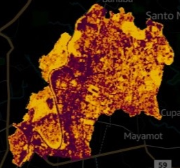
To visualize the predictions, Gramener used the SageMaker geospatial notebook with open-source geospatial libraries to overlay model predictions on a base map and provides layered visualize geospatial datasets directly within the notebook.

Conclusion

This post demonstrated how Gramener is empowering clients to make data-driven decisions for sustainable urban environments. With SageMaker, Gramener achieved substantial time savings in UHI analysis, reducing processing time from weeks to hours. This rapid insight generation allows Gramener’s clients to pinpoint areas requiring UHI mitigation strategies, proactively plan urban development and infrastructure projects to minimize UHI, and gain a holistic understanding of environmental factors for comprehensive risk assessment.

Discover the potential of integrating Earth observation data in your sustainability projects with SageMaker. For more information, refer to Get started with Amazon SageMaker geospatial capabilities.

About the Authors

Abhishek Mittal is a Solutions Architect for the worldwide public sector team with Amazon Web Services (AWS), where he primarily works with ISV partners across industries providing them with architectural guidance for building scalable architecture and implementing strategies to drive adoption of AWS services. He is passionate about modernizing traditional platforms and security in the cloud. Outside work, he is a travel enthusiast.

Janosch Woschitz is a Senior Solutions Architect at AWS, specializing in AI/ML. With over 15 years of experience, he supports customers globally in leveraging AI and ML for innovative solutions and building ML platforms on AWS. His expertise spans machine learning, data engineering, and scalable distributed systems, augmented by a strong background in software engineering and industry expertise in domains such as autonomous driving.

Shravan Kumar is a Senior Director of Client success at Gramener, with decade of experience in Business Analytics, Data Evangelism & forging deep Client Relations. He holds a solid foundation in Client Management, Account Management within the realm of data analytics, AI & ML.

Avirat S is a geospatial data scientist at Gramener, leveraging AI/ML to unlock insights from geographic data. His expertise lies in disaster management, agriculture, and urban planning, where his analysis informs decision-making processes.

• SEO Powered Content & PR Distribution. Get Amplified Today.
• PlatoData.Network Vertical Generative Ai. Empower Yourself. Access Here.
• PlatoAiStream. Web3 Intelligence. Knowledge Amplified. Access Here.
• PlatoESG. Carbon, CleanTech, Energy, Environment, Solar, Waste Management. Access Here.
• PlatoHealth. Biotech and Clinical Trials Intelligence. Access Here.
• Source: https://aws.amazon.com/blogs/machine-learning/understanding-and-predicting-urban-heat-islands-at-gramener-using-amazon-sagemaker-geospatial-capabilities/