Introduction
A reliable statistical technique for determining significance is the analysis of variance (ANOVA), especially when comparing more than two sample averages. Although the t-distribution is adequate for comparing the means of two samples, an ANOVA is required when working with three or more samples at once in order to determine whether or not their means are the same since they come from the same underlying population.
For example, ANOVA can be used to determine whether different fertilizers have different effects on wheat production in different plots and whether these treatments provide statistically different results from the same population.

Prof. R.A Fisher introduced the term ‘Analysis of Variance’ in 1920 when dealing with the problem in analysis of agronomical data. Variability is a fundamental feature of natural events. The overall variation in any given dataset originates from multiple sources, which can be broadly classified as assignable and chance causes.
The variation due to assignable causes can be detected and measured whereas the variation due to chance causes is beyond the control of human hand and cannot be treated separately.
According to R.A. Fisher, Analysis of Variance (ANOVA) is the “Separation of Variance ascribable to one group of causes from the variance ascribable to other group”.
Learning Objectives
- Understand the concept of Analysis of Variance (ANOVA) and its importance in statistical analysis, particularly when comparing multiple sample averages.
- Learn the assumptions required for conducting an ANOVA test and its application in different fields such as medicine, education, marketing, manufacturing, psychology, and agriculture.
- Explore the step-by-step process of performing a one-way ANOVA, including setting up null and alternative hypotheses, data collection and organization, calculation of group statistics, determination of sum of squares, computation of degrees of freedom, calculation of mean squares, computation of F-statistics, determination of critical value and decision making.
- Gain practical insights into implementing a one-way ANOVA test in Python using scipy.stats library.
- Understand the significance level and interpretation of the F-statistic and p-value in the context of ANOVA.
- Learn about post-hoc analysis methods like Tukey’s Honestly Significant Difference (HSD) for further analysis of significant differences among groups.
Table of contents
Assumptions for ANOVA TEST
ANOVA test is based on the test statistics F.
Assumptions made regarding the validity of the F-test in ANOVA include the following:
- The observations are independent.
- Parent population from which observations are taken is normal.
- Various treatment and environmental effects are additive in nature.
One-way ANOVA
One way ANOVA is a statistical test used to determine if there are statistically significant differences in the means of three or more groups for a single factor (independent variable). It compares the variance between groups to variance within groups to assess if these differences are likely due to random chance or a systematic effect of the factor.
Several use cases of one-way ANOVA from different domains are:
- Medicine: One-way ANOVA can be used to compare the effectiveness of different treatments on a particular medical condition. For example, it could be used to determine whether three different drugs have significantly different effects on reducing blood pressure.
- Education: One-way ANOVA can be used to analyze whether there are significant differences in test scores among students who have been taught using different teaching methods.
- Marketing: One-way ANOVA can be employed to assess whether there are significant differences in customer satisfaction levels among products from different brands.
- Manufacturing: One-way ANOVA can be utilized to analyze whether there are significant differences in the strength of materials produced by different manufacturing processes.
- Psychology: One-way ANOVA can be used to investigate whether there are significant differences in anxiety levels among participants exposed to different stressors.
- Agriculture: One-way ANOVA can be used to determine whether different fertilizers lead to significantly different crop yields in farming experiments.
Let’s understand this with Agriculture example in detail:
In agricultural research, one-way ANOVA can be employed to assess whether different fertilizers lead to significantly different crop yields.
Fertilizer Effect on Plant Growth
Imagine you are researching the impact of different fertilizers on plant growth. You apply three types of fertilizer (A, B and C) to separate groups of plants. After a set period, you measure the average height of plants in each group. You can use one-way ANOVA to test if there’s a significant difference in average height among plants grown with different fertilizers.
Step1: Null and Alternative Hypotheses
First step is to step up Null and Alternative Hypotheses:
- Null Hypothesis(H0): The means of all groups are equal (there’s no significant difference in plant growth due to fertilizer type)
- Alternative Hypothesis (H1): Atleast one group mean is different from the others (fertilizer type has a significant effect on plant growth).
Step2: Data Collection and Data Organization
After a set growth period, carefully measure the final height of each plant in all three groups. Now organize your data. Each column represents a fertilizer type (A, B, C) and each row holds the height of an individual plant within that group.
Step3: Calculate the group Statistics
- Compute the mean final height for plants in each fertilizer group (A, B and C).
- Compute the total number of plants observed (N) across all groups.
- Determine the total number of groups (K) in our case, k=3(A, B, C)
Step4: Calculate Sum of Square
So Total sum of square, between-group sum of square, within-group sum of square will be calculated.
Here, Total Sum of Square represents the total variation in final height across all plants.
Between-Group Sum of Square reflects the variation observed between the average heights of the three fertilizer groups. And Within-Group Sum of Square captures the variation in final heights within each fertilizer group.
Step5: Compute Degrees of Freedom
Degrees of freedom define the number of independent pieces of information used to estimate a population parameter.
- Degrees of Freedom Between-Group: k-1 (number of groups minus 1) So, here it will be 3-1 =2
- Degrees of Freedom Within-Group: N-k (Total number of observations minus number of groups)
Step6: Calculate Mean Squares
Mean Squares are obtained by dividing the respective Sum of Squares by degrees of freedom.
- Mean Square Between: Between- Group Sum of Square/Degrees of Freedom Between-Group
- Mean Square Within: Within-Group sum of Square/Degrees of Freedom Within-Group
Step7: Compute F-statistics
The F-statistic is a test statistic used to compare the variation between groups to the variation within groups. A higher F-statistic suggests a potentially stronger effect of fertilizer type on plant growth.
The F-statistic for one-way Anova is calculate by using this formula:
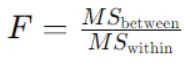
Here,
MSbetween is the mean square between groups, calculated as the sum of squares between groups divided by the degrees of freedom between groups.
MSwithin is the mean square within groups, calculated as the sum of squares within groups divided by the degrees of freedom within groups.
- Degrees of Freedom Between Groups(dof_between): dof_between = k-1
Where k is the number of groups(levels) of the independent variable.
- Degrees of Freedom Within Groups(dof_within): dof_within = N-k
Where N is the number of observations and k is the number of groups(levels) of the independent variable.
For one-way ANOVA, total degrees of freedom is the sum of the degrees of freedom between groups and within groups:
dof_total= dof_between+dof_within
Step8: Determine Critical Value and Decision
Choose a significance level (alpha) for the analysis, usually 0.05 is chosen
Look up the critical F-value at the chosen alpha level and the calculated Degrees of Freedom Between-Group and Degrees of Freedom Within-Group using an F-distribution table.
Compare the calculated F-statistic with the critical F-value
- If the calculated F-statistic is greater than the critical F-value, reject the null hypothesis(H0). This indicates a statistically significant difference in average plant heights among the three fertilizer groups.
- If the calculated F-statistic is less than or equal to the critical F-vale, fail to reject the null hypothesis (H0). You cannot conclude a significant difference based on this data.
Step9: Post-hoc Analysis (if necessary)
If the null hypothesis is rejected, signifying a significant overall difference, you might want to delve deeper. Post -hoc like Tukey’s Honestly Significant Difference (HSD) can help identify which specific fertilizer groups have statistically different average plant heights.
Implementation in Python:
import scipy.stats as stats

# Sample plant height data for each fertilizer type
plant_heights_A = [25, 28, 23, 27, 26]
plant_heights_B = [20, 22, 19, 21, 24]
plant_heights_C = [18, 20, 17, 19, 21]

# Perform one-way ANOVA
f_value, p_value = stats.f_oneway(plant_heights_A, plant_heights_B, plant_heights_C)

# Interpretation
print("F-statistic:", f_value)
print("p-value:", p_value)

# Significance level (alpha) - typically set at 0.05
alpha = 0.05

if p_value < alpha:
    print("Reject H0: There is a significant difference in plant growth between the fertilizer groups.")
else:
    print("Fail to reject H0: We cannot conclude a significant difference based on this sample.")
Output:

The degree of freedom between is K-1 = 3-1 =2 , where k represents the number of fertilizer groups. The degree of freedom within is N-k = 15-3= 12,, where N represents the total number of data points.
F-Critical at dof(2,12) can be calculated from F-Distribution table at 0.05 level of significance.
F-Critical = 9.42
Since F-Critical < F-statistics So, we reject the null hypothesis which concludes that there is significant difference in plant growth between the fertilizer groups.
With a p-value below 0.05, our conclusion remains consistent: we reject the null hypothesis, indicating a significant difference in plant growth among the fertilizer groups.
Two-way ANOVA
One-way ANOVA is suitable for only one factor, but what if you have two factors influencing your experiment? Then two -way ANOVA is used which allows you to analyze the effects of two independent variables on a single dependent variable.
Step1: Setting up Hypotheses
- Null hypothesis (H0): There’s no significant difference in average final plant height due to fertilizer type (A, B, C) or planting time (early, late) or their interaction.
- Alternative Hypothesis (H1): At least one the following is true:
- Fertilizer type has significant effect on average final height.
- Planting time has a significant effect on average final height.
- There’s a significant interaction effect between fertilizer type and planting time. This means the effect of one factor (fertilizer) depends on the level of the other factor (planting time).
Step2: Data Collection and Organization
- Measure final plant heights.
- Organize your data into a table with rows representing individual plants and columns for:
- Fertilizer type (A, B, C)
- Planting time (early, late)
- Final height(cm)
Here is the table:

Step3: Calculate Sum of Square
Similar to one-way ANOVA, you will have to calculate various sums of squares to assess the variation in final heights:
- Total Sum of Square (SST): Represents the total variation across all plants. Main effect sum of square:
- Between-Fertilizer Types (SSB_F): Reflects the variation due to differences in fertilizer type (averaged across planting times)
- Between-Plating Times (SSB_T): Reflects the variation due to differences in planting times (averaged across fertilizer types).
- Interaction sum of square (SSI): Captures the variation due to interaction between fertilizer type and planting time.
- Within-Group Sum of Squares (SSW): Represents the variation in final heights within each fertilizer-planting time combination.
Step4: Compute Degrees of Freedom (df):
Degrees of freedom define the number of independent pieces of information for each effect.
- dfTotal: N-1 (total observations minus 1)
- dfFertilizer: Number of fertilizer types -1
- dfPlanting Time: Number of planting times -1
- dfInteraction: (Number of fertilizer types -1) * (Number of planting times -1)
- dfWithin: dfTotal-dfFertilizer-dfplanting-dfInteraction
Step5: Calculate Mean Squares
Divide each Sum of Square by its corresponding degree of freedom.
- MS_Fertilizer: SSB_F/dfFertilizer
- MS_PlantingTime: SSB_T/dfPlanting
- MS_Interaction: SSI/dfInteraction
- MS_Within: SSW/dfWithin
Step6: Compute F-statistics
Calculate separate F-statistics for fertilizer type, planting time, and interaction effect:
- F_Fertilize: MS_Fertilizer/MS_Within
- F_PlantingTime: MS_PlantingTime/ MS_Within
- F_Interaction: MS_Inteaction/MS_Within
- F_PlantingTime: MS_PlantingTime/MS_Within
- F_Interaction: MS_Interaction/ MS_Within
Step7: Determine Critical Values and Decision:
Choose a significance level (alpha) for your analysis, usually we take 0.05
Look up critical F-values for each effect (fertilizer, planting time, interaction) at the chosen alpha level and their respective degrees of freedom using an F-distribution table or statistical software.
Compare your calculated F-statistics to the critical F-values for each effect:
- If the F-statistic is greater than the critical F-value, reject the null hypothesis(H0) for that effect. This indicates a statistically significant difference.
- If the F-statistic is less than or equal to the critical F-value fail to reject H0 for that effect. This indicates a statistically insignificant difference.
Step8: Post-hoc Analysis (if necessary)
If the null hypothesis is rejected, signifying a significant overall difference, you might want to delve deeper. Post -hoc like Tukey’s Honestly Significant Difference (HSD) can help identify which specific fertilizer groups have statistically different average plant heights.
import pandas as pd
import statsmodels.api as sm
from statsmodels.formula.api import ols
# Create a DataFrame from the dictionary
plant_heights = {
    'Treatment': ['A', 'A', 'A', 'A', 'A', 'A',
                  'B', 'B', 'B', 'B', 'B', 'B',
                  'C', 'C', 'C', 'C', 'C', 'C'],
    'Time': ['Early', 'Early', 'Early', 'Late', 'Late', 'Late',
             'Early', 'Early', 'Early', 'Late', 'Late', 'Late',
             'Early', 'Early', 'Early', 'Late', 'Late', 'Late'],
    'Height': [25, 28, 23, 27, 26, 24,
               20, 22, 19, 21, 24, 22,
               18, 20, 17, 19, 21, 20]
}
df = pd.DataFrame(plant_heights)


# Fit the ANOVA model
model = ols('Height ~ C(Treatment) + C(Time) + C(Treatment):C(Time)', data=df).fit()


# Perform ANOVA
anova_table = sm.stats.anova_lm(model, typ=2)


# Print the ANOVA table
print(anova_table)


# Interpret the results
alpha = 0.05  # Significance level

if anova_table['PR(>F)'][0] < alpha:
    print("nReject null hypothesis for Treatment factor.")
else:
    print("nFail to reject null hypothesis for Treatment factor.")

if anova_table['PR(>F)'][1] < alpha:
    print("Reject null hypothesis for Time factor.")
else:
    print("Fail to reject null hypothesis for Time factor.")

if anova_table['PR(>F)'][2] < alpha:
    print("Reject null hypothesis for Interaction between Treatment and Time.")
else:
    print("Fail to reject null hypothesis for Interaction between Treatment and Time.")
Output:
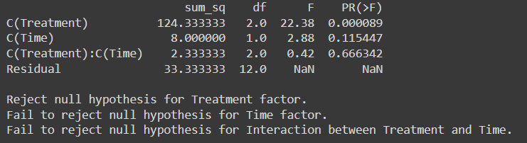
F-critical value for Treatment at degree of freedom (2,12) at 0.05 level of significance from F-distribution table is 9.42
F-critical value for Time at degree of freedom (1,12) at 0.05 level of significance is 61.22
F- critical value for interaction between treatment and Time at 0.05 level of significance at degree of freedom (2,12) is 9.42
Since F-Critical < F-statistics So, we reject the null hypothesis for Treatment Factor.
But for Time Factor and Interaction between Treatment and Time factor we failed to reject the Null Hypothesis as F-statistics value > F-Critical value
With a p-value below 0.05, our conclusion remains consistent: we reject the null hypothesis for Treatment Factor while with a p-value above 0.05 we fail to reject the Null hypothesis for Time factor and interaction between Treatment and Time factor.
Difference Between One- way ANOVA and TWO- way ANOVA
One-way ANOVA and Two-way ANOVA are both statistical techniques used to analyze differences among groups, but they differ in terms of the number of independent variables they consider and the complexity of the experimental design.
Here are the key differences between one-way ANOVA and two-way ANOVA:
| Aspect | One-way ANOVA | Two-way ANOVA |
|---|---|---|
| Number of Variables | Analyzes one independent variable (factor) on a continuous dependent variable | Analyzes two independent variables (factors) on a continuous dependent variable |
| Experimental Design | One categorical independent variable with multiple levels (groups) | Two categorical independent variables (factors), often labeled as A and B, with multiple levels. Allows examination of main effects and interaction effects |
| Interpretation | Indicates significant differences among group means | Provides info on main effects of factors (A and B) and their interaction. Helps assess differences between factor levels and interdependency |
| Complexity | Relatively straightforward and easy to interpret | More complex, analyzing main effects of two factors and their interaction. Requires careful consideration of factor relationships |
Conclusion
ANOVA is a powerful tool for analyzing differences among group means, essential when comparing more than two sample averages. One-way ANOVA assesses the impact of a single factor on a continuous outcome, while two-way ANOVA extends this analysis to consider two factors and their interaction effects. Understanding these differences enables researchers to choose the most suitable analytical approach for their experimental designs and research questions.
Frequently Asked Questions
A. ANOVA stands for Analysis of Variance, a statistical method used to analyze differences among group means. It is used when comparing means across three or more groups to determine if there are significant differences.
A. One-way ANOVA is used when you have one categorical independent variable (factor) with multiple levels and you want to compare the means of these levels. For example, comparing the effectiveness of different treatments on a single outcome.
A. Two-way ANOVA is used when you have two categorical independent variables (factors) and you want to analyze their effects on a continuous dependent variable, as well as the interaction between the two factors. It’s useful for studying the combined effects of two factors on an outcome.
A. The p-value in ANOVA indicates the probability of observing the data if the null hypothesis (no significant difference among group means) were true. A low p-value (< 0.05) suggests that there is significant evidence to reject the null hypothesis and conclude that there are differences among the groups.)
A. The F-statistic in ANOVA measures the ratio of the variance between groups to the variance within groups. A higher F-statistic indicates that the variance between groups is larger relative to the variance within groups, suggesting a significant difference among the group means.
- SEO Powered Content & PR Distribution. Get Amplified Today.
- PlatoData.Network Vertical Generative Ai. Empower Yourself. Access Here.
- PlatoAiStream. Web3 Intelligence. Knowledge Amplified. Access Here.
- PlatoESG. Carbon, CleanTech, Energy, Environment, Solar, Waste Management. Access Here.
- PlatoHealth. Biotech and Clinical Trials Intelligence. Access Here.
- Source: https://www.analyticsvidhya.com/blog/2024/04/one-way-and-two-way-analysis-of-variance-anova/

