
Image by OrMaVaredo on Pixabay
Python is one of the most used programming languages in the world and provides developers with a wide range of libraries.
Anyway, when it comes to data manipulation and scientific computation, we generally think of libraries such as Numpy, Pandas, or SciPy.
In this article, we introduce 3 Python libraries you may be interested in.
Introducing Dask
Dask is a flexible parallel computing library that enables distributed computing and parallelism for large-scale data processing.
So, why should we use Dask? As they say on their website:
Python has grown to become the dominant language both in data analytics and general programming. This growth has been fueled by computational libraries like NumPy, pandas, and scikit-learn. However, these packages weren’t designed to scale beyond a single machine. Dask was developed to natively scale these packages and the surrounding ecosystem to multi-core machines and distributed clusters when datasets exceed memory.
So, one of the common uses of Dask, as they say, is:
Dask DataFrame is used in situations where pandas is commonly needed, usually when pandas fails due to data size or computation speed:
– Manipulating large datasets, even when those datasets don’t fit in memory
– Accelerating long computations by using many cores
– Distributed computing on large datasets with standard pandas operations like groupby, join, and time series computations
So, Dask is a good choice when we need to deal with huge Pandas data frames. This is because Dask:
Allows users to manipulate 100GB+ datasets on a laptop or 1TB+ datasets on a workstation
Which is a pretty impressive result.
What happens under the hood, is that:
Dask DataFrames coordinate many pandas DataFrames/Series arranged along the index. A Dask DataFrame is partitioned row-wise, grouping rows by index value for efficiency. These pandas objects may live on disk or on other machines.
So, we have something like that:
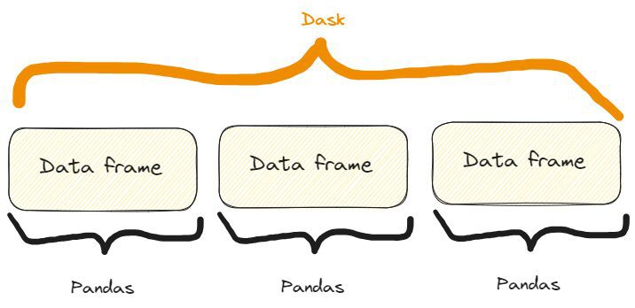
The difference between a Dask and a Pandas data frame. Image by Author, freely inspired by one on the Dask website already quoted.
Some features of Dask in action
First of all, we need to install Dask. We can do it via pip or conda like so:
$ pip install dask[complete] or $ conda install daskFEATURE ONE: OPENING A CSV FILE
The first feature we can show of Dask is how we can open a CSV. We can do it like so:
import dask.dataframe as dd # Load a large CSV file using Dask
df_dask = dd.read_csv('my_very_large_dataset.csv') # Perform operations on the Dask DataFrame
mean_value_dask = df_dask['column_name'].mean().compute()
So, as we can see in the code, the way we use Dask is very similar to Pandas. In particular:
- We use the method
read_csv()exactly as in Pandas - We intercept a column exactly as in Pandas. In fact, if we had a Pandas data frame called
dfwe’d intercept a column this way:df['column_name']. - We apply the
mean()method to the intercepted column similar to Pandas, but here we also need to add the methodcompute().
Also, even if the methodology of opening a CSV file it’s the same as in Pandas, under the hood Dask is effortlessly processing a large dataset that exceeds the memory capacity of a single machine.
This means that we can’t see any actual difference, except the fact that a large data frame can’t be opened in Pandas, but in Dask we can.
FEATURE TWO: SCALING MACHINE LEARNING WORKFLOWS
We can use Dask to also create a classification dataset with a huge number of samples. We can then split it into the train and the test sets, fit the train set with an ML model, and calculate predictions for the test set.
We can do it like so:
import dask_ml.datasets as dask_datasets
from dask_ml.linear_model import LogisticRegression
from dask_ml.model_selection import train_test_split # Load a classification dataset using Dask
X, y = dask_datasets.make_classification(n_samples=100000, chunks=1000) # Split the data into train and test sets
X_train, X_test, y_train, y_test = train_test_split(X, y) # Train a logistic regression model in parallel
model = LogisticRegression()
model.fit(X_train, y_train) # Predict on the test set
y_pred = model.predict(X_test).compute()
This example stresses the ability of Dask to handle huge datasets even in the case of a Machine Learning problem, by distributing computations across multiple cores.
In particular, we can create a “Dask dataset” for a classification case with the method dask_datasets.make_classification(), and we can specify the number of samples and chunks (even, very huge!).
Similarly as before, the predictions are obtained with the method compute().
NOTE: in this case, you may need to intsall the module dask_ml. You can do it like so: $ pip install dask_mlFEATURE THREE: EFFICIENT IMAGE PROCESSING
The power of parallel processing that Dask utilizes can also be applied to images.
In particular, we could open multiple images, resize them, and save them resized. We can do it like so:
import dask.array as da
import dask_image.imread
from PIL import Image # Load a collection of images using Dask
images = dask_image.imread.imread('image*.jpg') # Resize the images in parallel
resized_images = da.stack([da.resize(image, (300, 300)) for image in images]) # Compute the result
result = resized_images.compute() # Save the resized images
for i, image in enumerate(result): resized_image = Image.fromarray(image) resized_image.save(f'resized_image_{i}.jpg')
So, here’s the process:
- We open all the “.jpg” images in the current folder (or in a folder that you can specify) with the method
dask_image.imread.imread("image*.jpg"). - We resize them all at 300×300 using a list comprehension in the method
da.stack(). - We compute the result with the method
compute(), as we did before. - We save all the resized images with the for cycle.
Introducing Sympy
If you need to make mathematical calculations and computations and want to stick to Python, you can try Sympy.
Indeed: why use other tools and software, when we can use our beloved Python?
As per what they write on their website, Sympy is:
A Python library for symbolic mathematics. It aims to become a full-featured computer algebra system (CAS) while keeping the code as simple as possible in order to be comprehensible and easily extensible. SymPy is written entirely in Python.
But why use SymPy? They suggest:
SymPy is…
– Free: Licensed under BSD, SymPy is free both as in speech and as in beer.
– Python-based: SymPy is written entirely in Python and uses Python for its language.
– Lightweight: SymPy only depends on mpmath, a pure Python library for arbitrary floating point arithmetic, making it easy to use.
– A library: Beyond use as an interactive tool, SymPy can be embedded in other applications and extended with custom functions.
So, it basically has all the characteristics that can be loved by Python addicts!
Now, let’s see some of its features.
Some features of SymPy in action
First of all, we need to install it:
$ pip install sympyPAY ATTENTION: if you write $ pip install simpy you'll install another (completely different!) library. So, the second letter is a "y", not an "i".FEATURE ONE: SOLVING AN ALGEBRAIC EQUATION
If we need to solve an algebraic equation, we can use SymPy like so:
from sympy import symbols, Eq, solve # Define the symbols
x, y = symbols('x y') # Define the equation
equation = Eq(x**2 + y**2, 25) # Solve the equation
solutions = solve(equation, (x, y)) # Print solution
print(solutions) >>> [(-sqrt(25 - y**2), y), (sqrt(25 - y**2), y)]
So, that’s the process:
- We define the symbols of the equation with the method
symbols(). - We write the algebraic equation with the method
Eq. - We solve the equation with the method
solve().
When I was at the University I used different tools to solve these kinds of problems, and I have to say that SymPy, as we can see, is very readable and user-friendly.
But, indeed: it’s a Python library, so how could that be any different?
FEATURE TWO: CALCULATING DERIVATIVES
Calculating derivatives is another task we may mathematically need, for a lot of reasons when analyzing data. Often, we may need calculations for any reason, and SympY really simplifies this process. In fact, we can do it like so:
from sympy import symbols, diff # Define the symbol
x = symbols('x') # Define the function
f = x**3 + 2*x**2 + 3*x + 4 # Calculate the derivative
derivative = diff(f, x) # Print derivative
print(derivative) >>> 3*x**2 + 4*x + 3
So, as we can see, the process is very simple and self-explainable:
- We define the symbol of the function we’re deriving with
symbols(). - We define the function.
- We calculate the derivative with
diff()specifying the function and the symbol we’re calculating the derivative (this is an absolute derivative, but we could perform even partial derivatives in the case of functions that havexandyvariables).
And if we test it, we’ll see that the result arrives in a matter of 2 or 3 seconds. So, it’s also pretty fast.
FEATURE THREE: CALCULATING INTEGRATIONS
Of course, if SymPy can calculate derivatives, it can also calculate integrations. Let’s do it:
from sympy import symbols, integrate, sin # Define the symbol
x = symbols('x') # Perform symbolic integration
integral = integrate(sin(x), x) # Print integral
print(integral) >>> -cos(x)
So, here we use the method integrate(), specifying the function to integrate and the variable of integration.
Couldn’t it be easier?!
Introducing Xarray
Xarray is a Python library that extends the features and functionalities of NumPy, giving us the possibility to work with labeled arrays and datasets.
As they say on their website, in fact:
Xarray makes working with labeled multi-dimensional arrays in Python simple, efficient, and fun!
And also:
Xarray introduces labels in the form of dimensions, coordinates and attributes on top of raw NumPy-like multidimensional arrays, which allows for a more intuitive, more concise, and less error-prone developer experience.
In other words, it extends the functionality of NumPy arrays by adding labels or coordinates to the array dimensions. These labels provide metadata and enable more advanced analysis and manipulation of multi-dimensional data.
For example, in NumPy, arrays are accessed using integer-based indexing.
In Xarray, instead, each dimension can have a label associated with it, making it easier to understand and manipulate the data based on meaningful names.
For example, instead of accessing data with arr[0, 1, 2], we can use arr.sel(x=0, y=1, z=2) in Xarray, where x, y, and z are dimension labels.
This makes the code much more readable!
So, let’s see some features of Xarray.
Some features of Xarray in action
As usual, to install it:
$ pip install xarrayFEATURE ONE: WORKING WITH LABELED COORDINATES
Suppose we want to create some data related to temperature and we want to label these with coordinates like latitude and longitude. We can do it like so:
import xarray as xr
import numpy as np # Create temperature data
temperature = np.random.rand(100, 100) * 20 + 10 # Create coordinate arrays for latitude and longitude
latitudes = np.linspace(-90, 90, 100)
longitudes = np.linspace(-180, 180, 100) # Create an Xarray data array with labeled coordinates
da = xr.DataArray( temperature, dims=['latitude', 'longitude'], coords={'latitude': latitudes, 'longitude': longitudes}
) # Access data using labeled coordinates
subset = da.sel(latitude=slice(-45, 45), longitude=slice(-90, 0))
And if we print them we get:
# Print data
print(subset) >>>

array([[13.45064786, 29.15218061, 14.77363206, ..., 12.00262833, 16.42712411, 15.61353963], [23.47498117, 20.25554247, 14.44056286, ..., 19.04096482, 15.60398491, 24.69535367], [25.48971105, 20.64944534, 21.2263141 , ..., 25.80933737, 16.72629302, 29.48307134], ..., [10.19615833, 17.106716 , 10.79594252, ..., 29.6897709 , 20.68549602, 29.4015482 ], [26.54253304, 14.21939699, 11.085207 , ..., 15.56702191, 19.64285595, 18.03809074], [26.50676351, 15.21217526, 23.63645069, ..., 17.22512125, 13.96942377, 13.93766583]])
Coordinates: * latitude (latitude) float64 -44.55 -42.73 -40.91 ... 40.91 42.73 44.55 * longitude (longitude) float64 -89.09 -85.45 -81.82 ... -9.091 -5.455 -1.818
So, let’s see the process step-by-step:
- We’ve created the temperature values as a NumPy array.
- We’ve defined the latitudes and longitueas values as NumPy arrays.
- We’ve stored all the data in an Xarray array with the method
DataArray(). - We’ve selected a subset of the latitudes and longitudes with the method
sel()that selects the values we want for our subset.
The result is also easily readable, so labeling is really helpful in a lot of cases.
FEATURE TWO: HANDLING MISSING DATA
Suppose we’re collecting data related to temperatures during the year. We want to know if we have some null values in our array. Here’s how we can do so:
import xarray as xr
import numpy as np
import pandas as pd # Create temperature data with missing values
temperature = np.random.rand(365, 50, 50) * 20 + 10
temperature[0:10, :, :] = np.nan # Set the first 10 days as missing values # Create time, latitude, and longitude coordinate arrays
times = pd.date_range('2023-01-01', periods=365, freq='D')
latitudes = np.linspace(-90, 90, 50)
longitudes = np.linspace(-180, 180, 50) # Create an Xarray data array with missing values
da = xr.DataArray( temperature, dims=['time', 'latitude', 'longitude'], coords={'time': times, 'latitude': latitudes, 'longitude': longitudes}
) # Count the number of missing values along the time dimension
missing_count = da.isnull().sum(dim='time') # Print missing values
print(missing_count) >>>
array([[10, 10, 10, ..., 10, 10, 10], [10, 10, 10, ..., 10, 10, 10], [10, 10, 10, ..., 10, 10, 10], ..., [10, 10, 10, ..., 10, 10, 10], [10, 10, 10, ..., 10, 10, 10], [10, 10, 10, ..., 10, 10, 10]])
Coordinates: * latitude (latitude) float64 -90.0 -86.33 -82.65 ... 82.65 86.33 90.0 * longitude (longitude) float64 -180.0 -172.7 -165.3 ... 165.3 172.7 180.0
And so we obtain that we have 10 null values.
Also, if we take a look closely at the code, we can see that we can apply Pandas’ methods to an Xarray like isnull.sum(), as in this case, that counts the total number of missing values.
FEATURE ONE: HANDLING AND ANALYZING MULTI-DIMENSIONAL DATA
The temptation to handle and analyze multi-dimensional data is high when we have the possibility to label our arrays. So, why not try it?
For example, suppose we’re still collecting data related to temperatures at certain latitudes and longitudes.
We may want to calculate the mean, the max, and the median temperatures. We can do it like so:
import xarray as xr
import numpy as np
import pandas as pd # Create synthetic temperature data
temperature = np.random.rand(365, 50, 50) * 20 + 10 # Create time, latitude, and longitude coordinate arrays
times = pd.date_range('2023-01-01', periods=365, freq='D')
latitudes = np.linspace(-90, 90, 50)
longitudes = np.linspace(-180, 180, 50) # Create an Xarray dataset
ds = xr.Dataset( { 'temperature': (['time', 'latitude', 'longitude'], temperature), }, coords={ 'time': times, 'latitude': latitudes, 'longitude': longitudes, }
) # Perform statistical analysis on the temperature data
mean_temperature = ds['temperature'].mean(dim='time')
max_temperature = ds['temperature'].max(dim='time')
min_temperature = ds['temperature'].min(dim='time') # Print values print(f"mean temperature:n {mean_temperature}n")
print(f"max temperature:n {max_temperature}n")
print(f"min temperature:n {min_temperature}n") >>> mean temperature:
array([[19.99931701, 20.36395016, 20.04110699, ..., 19.98811842, 20.08895803, 19.86064693], [19.84016491, 19.87077812, 20.27445405, ..., 19.8071972 , 19.62665953, 19.58231185], [19.63911165, 19.62051976, 19.61247548, ..., 19.85043831, 20.13086891, 19.80267099], ..., [20.18590514, 20.05931149, 20.17133483, ..., 20.52858247, 19.83882433, 20.66808513], [19.56455575, 19.90091128, 20.32566232, ..., 19.88689221, 19.78811145, 19.91205212], [19.82268297, 20.14242279, 19.60842148, ..., 19.68290006, 20.00327294, 19.68955107]])
Coordinates: * latitude (latitude) float64 -90.0 -86.33 -82.65 ... 82.65 86.33 90.0 * longitude (longitude) float64 -180.0 -172.7 -165.3 ... 165.3 172.7 180.0 max temperature:
array([[29.98465531, 29.97609171, 29.96821276, ..., 29.86639343, 29.95069558, 29.98807808], [29.91802049, 29.92870312, 29.87625447, ..., 29.92519055, 29.9964299 , 29.99792388], [29.96647016, 29.7934891 , 29.89731136, ..., 29.99174546, 29.97267052, 29.96058079], ..., [29.91699117, 29.98920555, 29.83798369, ..., 29.90271746, 29.93747041, 29.97244906], [29.99171911, 29.99051943, 29.92706773, ..., 29.90578739, 29.99433847, 29.94506567], [29.99438621, 29.98798699, 29.97664488, ..., 29.98669576, 29.91296382, 29.93100249]])
Coordinates: * latitude (latitude) float64 -90.0 -86.33 -82.65 ... 82.65 86.33 90.0 * longitude (longitude) float64 -180.0 -172.7 -165.3 ... 165.3 172.7 180.0 min temperature:
array([[10.0326431 , 10.07666029, 10.02795524, ..., 10.17215336, 10.00264909, 10.05387097], [10.00355858, 10.00610942, 10.02567816, ..., 10.29100316, 10.00861792, 10.16955806], [10.01636216, 10.02856619, 10.00389027, ..., 10.0929342 , 10.01504103, 10.06219179], ..., [10.00477003, 10.0303088 , 10.04494723, ..., 10.05720692, 10.122994 , 10.04947012], [10.00422182, 10.0211205 , 10.00183528, ..., 10.03818058, 10.02632697, 10.06722953], [10.10994581, 10.12445222, 10.03002468, ..., 10.06937041, 10.04924046, 10.00645499]])
Coordinates: * latitude (latitude) float64 -90.0 -86.33 -82.65 ... 82.65 86.33 90.0 * longitude (longitude) float64 -180.0 -172.7 -165.3 ... 165.3 172.7 180.0
And we obtained what we wanted, also in a clearly readable way.
And again, as before, to calculate the max, min, and mean values of temperatures we’ve used Pandas’ functions applied to an array.
In this article, we’ve shown three libraries for scientific calculation and computation.
While SymPy can be the substitute for other tools and software, giving us the possibility to use Python code to compute mathematical calculations, Dask and Xarray extend the functionalities of other libraries, helping us in situations where we may have difficulties with other most known Python libraries for data analysis and manipulation.
Federico Trotta has loved writing since he was a young boy in school, writing detective stories as class exams. Thanks to his curiosity, he discovered programming and AI. Having a burning passion for writing, he couldn’t avoid starting to write about these topics, so he decided to change his career to become a Technical Writer. His purpose is to educate people on Python programming, Machine Learning, and Data Science, through writing. Find more about him at federicotrotta.com.
Original. Reposted with permission.
- SEO Powered Content & PR Distribution. Get Amplified Today.
- PlatoData.Network Vertical Generative Ai. Empower Yourself. Access Here.
- PlatoAiStream. Web3 Intelligence. Knowledge Amplified. Access Here.
- PlatoESG. Automotive / EVs, Carbon, CleanTech, Energy, Environment, Solar, Waste Management. Access Here.
- PlatoHealth. Biotech and Clinical Trials Intelligence. Access Here.
- ChartPrime. Elevate your Trading Game with ChartPrime. Access Here.
- BlockOffsets. Modernizing Environmental Offset Ownership. Access Here.
- Source: https://www.kdnuggets.com/2023/08/beyond-numpy-pandas-unlocking-potential-lesserknown-python-libraries.html?utm_source=rss&utm_medium=rss&utm_campaign=beyond-numpy-and-pandas-unlocking-the-potential-of-lesser-known-python-libraries

