Image by Author
Predicting the future isn’t magic; it’s an AI.
As we stand on the brink of the AI revolution, Python allows us to participate.
In this one, we’ll discover how you can use Python and Machine Learning to make predictions.
We’ll start with real fundamentals and go to the place where we’ll apply algorithms to the data to make a prediction. Let’s get started!
What is Machine Learning?
Machine learning is a way of giving the computer the ability to make predictions. It is too popular now; you probably use it daily without noticing. Here are some technologies that are benefitting from Machine Learning;
- Self Driving Cars
- Face Detection System
- Netflix Movie Recommendation System
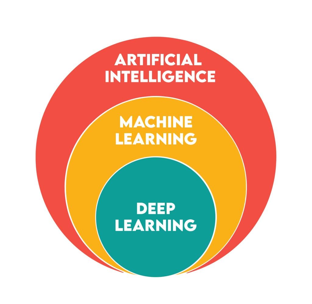
But sometimes, AI & Machine Learning, and Deep learning can not be distinguished well.
Here is a grand scheme that best represents those terms.
Classifying Machine Learning As a Beginner
Machine Learning algorithms can be clustered by using two different methods. One of these methods involves determining whether a ‘label’ is associated with the data points. In this context, a ‘label’ refers to the specific attribute or characteristic of the data points you want to predict.
If there is a label, your algorithm is classified as a supervised algorithm; otherwise, it is an unsupervised algorithm.
Another method to classify machine learning algorithms is classifying the algorithm. If you do that, machine learning algorithms can be clustered as follows:
Like Sci-kit Learn did, here.
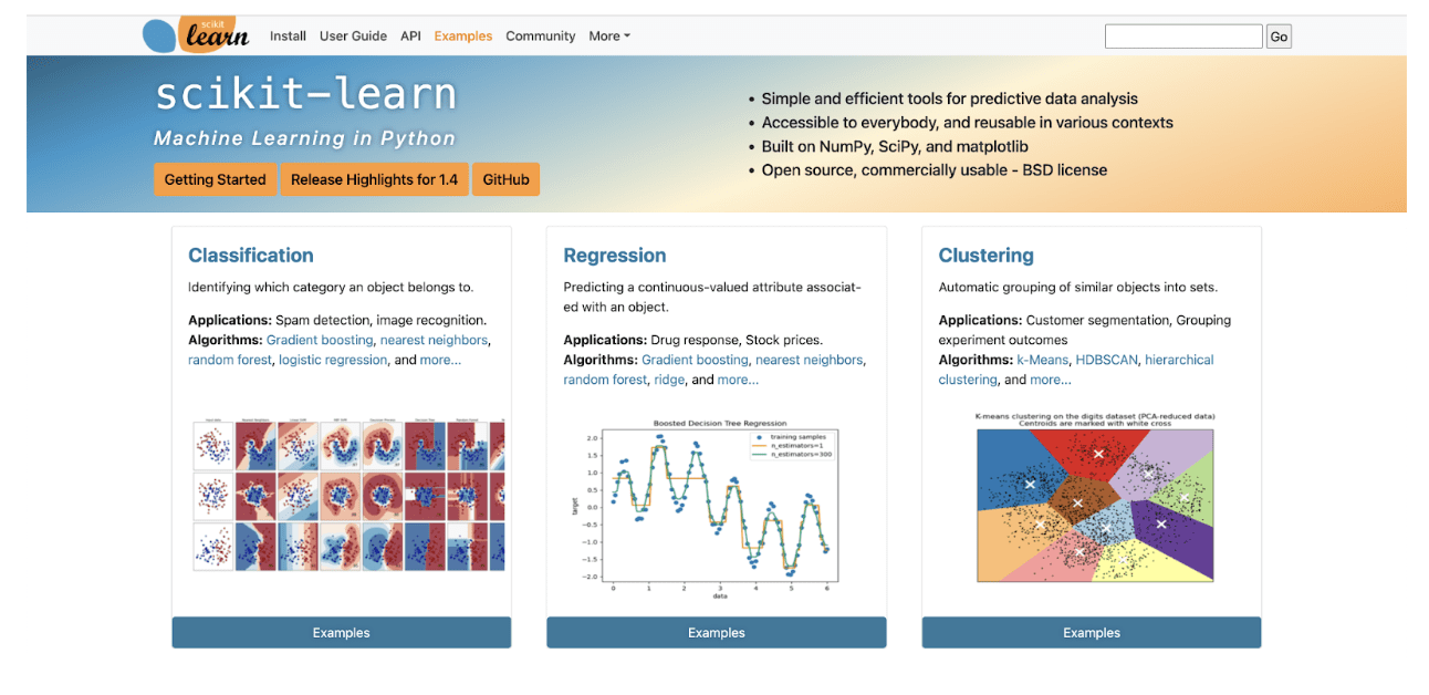
Image source: scikit-learn.org
What is Sci-kit Learn?
Sci-kit learn is the most famous machine learning library in Python; we’ll use this in this article. Using Sci-kit Learn, you will skip defining algorithms from scratch and use the built-in functions from Sci-kit Learn, which will ease your way of building machine learning.
In this article, we’ll build a machine-learning model using different regression algorithms from the sci-kit Learn. Let’s first explain regression.
What is Regression?
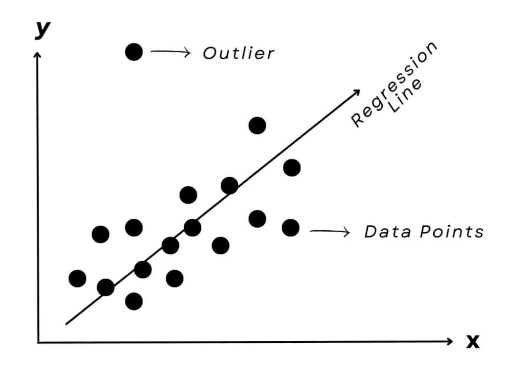
Regression is a machine learning algorithm that makes predictions about continuous value. Here are some real-life examples of regression,
Now, before applying Regression models, let’s see three different regression algorithms with simple explanations;
- Multiple Linear Regression: Predicts using a linear combination of multiple predictor variables.
- Decision Tree Regressor: Creates a tree-like model of decisions to predict the value of a target variable based on several input features.
- Support Vector Regression: Finds the best-fit line (or hyperplane in higher dimensions) with the maximum number of points within a certain distance.
Before applying machine learning, you need to follow specific steps. Sometimes, these steps might differ; however, most of the time, they include;
- Data Exploration and Analysis
- Data Manipulation
- Train-test split
- Building ML Model
- Data Visualization
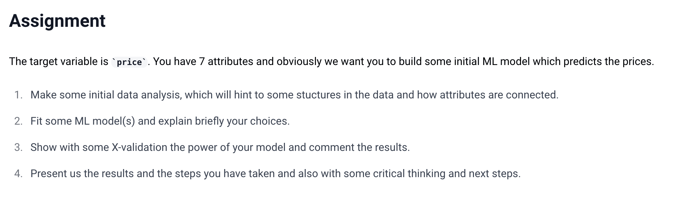
In this one, let’s use a data project from our platform to predict price here.
Data Exploration and Analysis
In Python, we have several functions. By using them, you can become acquainted with the data you use.
But first of all, you should load the libraries with these functions.
import pandas as pd
import sklearn
from sklearn.linear_model import LinearRegression
from sklearn.ensemble import RandomForestRegressor
from sklearn import svm
from sklearn.model_selection import train_test_split
from sklearn.metrics import r2_score
from sklearn.metrics import mean_squared_error
Excellent, let’s load our data and explore it a little bit
data = pd.read_csv('path')Input the path of the file in your directory. Python has three functions that will help you explore the data. Let’s apply them one by one and see the result.
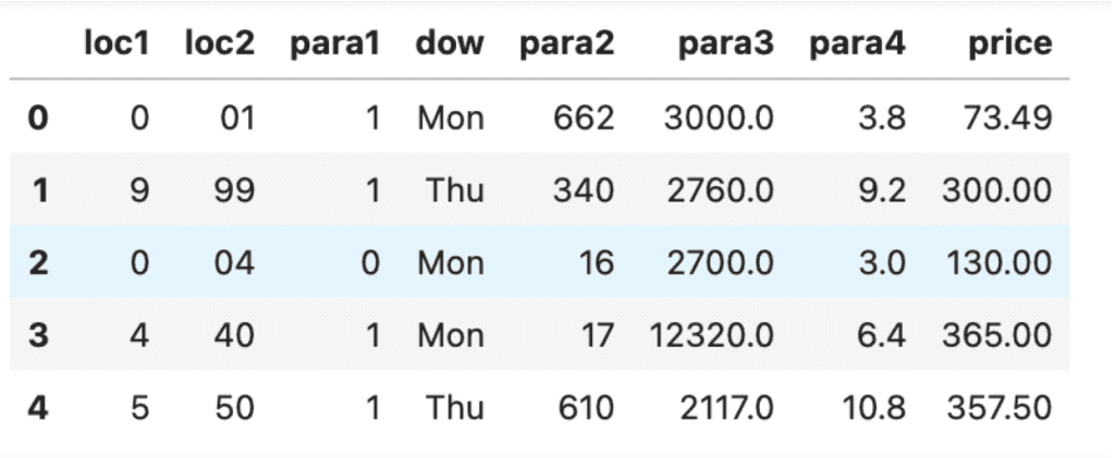
Here is the code to see the first five rows of our dataset.
data.head()Here is the output.
Now, let’s examine our second function: view the information about our datasets column.
data.info()Here is the output.
RangeIndex: 10000 entries, 0 to 9999
Data columns (total 8 columns):
  #     Column     Non-Null  Count   Dtype
- - -   - - - -    - - - - - - - -   - - - -
  0     loc1       10000 non-null     object
  1     loc2       10000 non-null     object
  2     para1      10000 non-null     int64
  3     dow        10000 non-null     object
  4     para2      10000 non-null     int64
  5     para3      10000 non-null     float64
  6     para4      10000 non-null     float64
  7     price      10000 non-null     float64
 dtypes:   float64(3),   int64(2),   object(3)
 memory  usage:  625.1+ KB
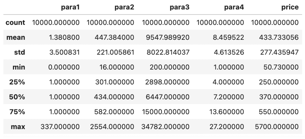
Here is the last function, which will summarize our data statistically. Here is the code.
data.describe()Here is the output.
Now, you are more familiar with our data. In machine learning, all your predictor variables, which means the columns you intend to use to make a prediction, should be numerical.
In the next section, we’ll make sure about it.
Data Manipulation
Now, we all know that we should convert the “dow” column to numbers, but before that, let’s check if other columns consist of numbers only for the sake of our machine-learning models.
We have two suspected columns, loc1, and loc2, because, as you can see from the output of the info() function, we have just two columns that are object data types, which can include numerical and string values.
Let’s use this code to check;
data["loc1"].value_counts()Here is the output.
loc1
2	1607
0	1486
1	1223
7	1081
3	945
5	846
4	773
8	727
9	690
6	620
S	  1
T	  1
Name:  count,  dtype:  int64
Now, by using the following code, you can eliminate those rows.
data = data[(data["loc1"] != "S") & (data["loc1"] != "T")]However, we must ensure that the other column, loc2, does not contain string values. Let’s use the following code to ensure that all values are numerical.
data["loc2"] = pd.to_numeric(data["loc2"], errors='coerce')
data["loc1"] = pd.to_numeric(data["loc1"], errors='coerce')
data.dropna(inplace=True)
At the end of the code above, we use the dropna() function because the converting function from pandas will convert “na” to non-numerical values.
Excellent. We can solve this issue; let’s convert weekday columns into numbers. Here is the code to do that;
# Assuming data is already loaded and 'dow' column contains day names
# Map 'dow' to numeric codes
days_of_week = {'Mon': 1, 'Tue': 2, 'Wed': 3, 'Thu': 4, 'Fri': 5, 'Sat': 6, 'Sun': 7}
data['dow'] = data['dow'].map(days_of_week)
# Invert the days_of_week dictionary
week_days = {v: k for k, v in days_of_week.items()}
# Convert dummy variable columns to integer type
dow_dummies = pd.get_dummies(data['dow']).rename(columns=week_days).astype(int)
# Drop the original 'dow' column
data.drop('dow', axis=1, inplace=True)
# Concatenate the dummy variables
data = pd.concat([data, dow_dummies], axis=1)
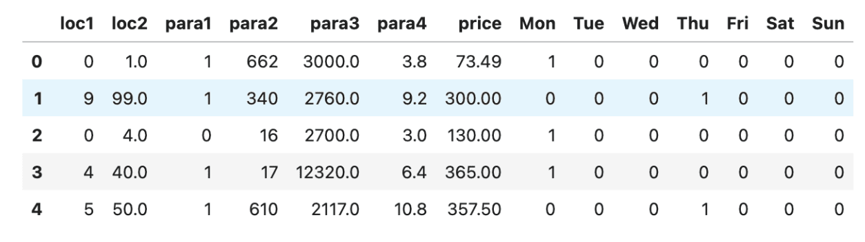
data.head()
In this code, we define weekdays by defining a number for each day in the dictionary and then simply changing the day names with those numbers. Here is the output.
Now, we are almost there.
Train-Test Split
Before applying a machine learning model, you must split your data into training and test sets. This allows you to objectively assess your model’s efficiency by training it on the training set and then evaluating its performance on the test set, which the model has not seen before.
X = data.drop('price', axis=1)  # Assuming 'price' is the target variable
y = data['price']
X_train, X_test, y_train, y_test = train_test_split(X, y, test_size=0.2, random_state=42)
Building Machine Learning Model
Now everything is ready. At this stage, we’ll apply the following algorithms at once.
- Multiple Linear Regression
- Decision Tree Regression
- Support Vector Regression
If you are a beginner, this code might seem complicated, but rest assured, it is not. In the code, we first assign model names and their corresponding functions from scikit-learn to the model’s dictionary.
Next, we create an empty dictionary called results to store these results. In the first loop, we simultaneously apply all the machine learning models and evaluate them using metrics such as R^2 and MSE, which assess how well the algorithms perform.
In the final loop, we print out the results that we have saved. Here is the code
# Initialize the models
models = {
    "Multiple Linear Regression": LinearRegression(),
    "Decision Tree Regression": DecisionTreeRegressor(random_state=42),
    "Support Vector Regression": SVR()
}

# Dictionary to store the results
results = {}

# Fit the models and evaluate
for name, model in models.items():
    model.fit(X_train, y_train)  # Train the model
    y_pred = model.predict(X_test)  # Predict on the test set

    # Calculate performance metrics
    mse = mean_squared_error(y_test, y_pred)
    r2 = r2_score(y_test, y_pred)

    # Store results
    results[name] = {'MSE': mse, 'R^2 Score': r2}

# Print the results
for model_name, metrics in results.items():
    print(f"{model_name} - MSE: {metrics['MSE']}, R^2 Score: {metrics['R^2 Score']}")
Here is the output.
Multiple Linear Regression - MSE: 35143.23011545407, R^2 Score: 0.5825954700994046
Decision Tree Regression - MSE: 44552.00644904675, R^2 Score: 0.4708451884787034
Support Vector Regression - MSE: 73965.02477382126, R^2 Score: 0.12149975134965318
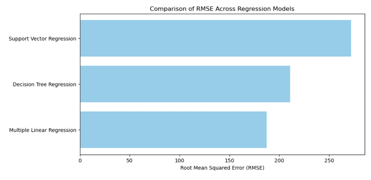
Data Visualization
To see the results better, let’s visualize the output.
Here is the code where we first calculate RMSE (square root of MSE) and visualize the output.
import matplotlib.pyplot as plt
from math import sqrt

# Calculate RMSE for each model from the stored MSE and prepare for plotting
rmse_values = [sqrt(metrics['MSE']) for metrics in results.values()]
model_names = list(results.keys())

# Create a horizontal bar graph for RMSE
plt.figure(figsize=(10, 5))
plt.barh(model_names, rmse_values, color='skyblue')
plt.xlabel('Root Mean Squared Error (RMSE)')
plt.title('Comparison of RMSE Across Regression Models')
plt.show()
Here is the output.
Data Projects
Before wrapping up, here are a few data projects to start.
Also, if you want to do data projects about interesting datasets, here are a few datasets that might become interesting to you;
Conclusion
Our results could be better because too many steps exist to improve the model’s efficiency, but we made a great start here. Check out Sci-kit Learn’s official document to see what you can do more.
Of course, after learning, you need to do data projects repeatedly to improve your capabilities and learn a few more things.
Nate Rosidi is a data scientist and in product strategy. He’s also an adjunct professor teaching analytics, and is the founder of StrataScratch, a platform helping data scientists prepare for their interviews with real interview questions from top companies. Nate writes on the latest trends in the career market, gives interview advice, shares data science projects, and covers everything SQL.
- SEO Powered Content & PR Distribution. Get Amplified Today.
- PlatoData.Network Vertical Generative Ai. Empower Yourself. Access Here.
- PlatoAiStream. Web3 Intelligence. Knowledge Amplified. Access Here.
- PlatoESG. Carbon, CleanTech, Energy, Environment, Solar, Waste Management. Access Here.
- PlatoHealth. Biotech and Clinical Trials Intelligence. Access Here.
- Source: https://www.kdnuggets.com/beginners-guide-to-machine-learning-with-python?utm_source=rss&utm_medium=rss&utm_campaign=beginners-guide-to-machine-learning-with-python

