작성자 별 이미지
Scikit-learn 파이프라인을 사용하면 전처리 및 모델링 단계를 단순화하고, 코드 복잡성을 줄이고, 데이터 전처리의 일관성을 보장하고, 하이퍼파라미터 조정을 지원하고, 워크플로를 더욱 체계화하고 유지 관리하기 쉽게 만들 수 있습니다. 파이프라인은 여러 변환과 최종 모델을 단일 엔터티로 통합하여 재현성을 향상하고 모든 것을 더욱 효율적으로 만듭니다.
이 튜토리얼에서 우리는 은행 이탈 Random Forest Classifier를 훈련하기 위한 Kaggle의 데이터 세트입니다. 데이터 전처리 및 모델 교육의 기존 접근 방식을 Scikit-learn 파이프라인 및 ColumnTransformers를 사용하는 보다 효율적인 방법과 비교할 것입니다.
데이터 처리 파이프라인에서는 범주형 열과 숫자형 열을 개별적으로 변환하는 방법을 알아봅니다. 우리는 전통적인 스타일의 코드로 시작한 다음 유사한 처리를 수행하는 더 나은 방법을 보여줄 것입니다.
zip 파일에서 데이터를 추출한 후 인덱스 열이 "id"인 `train.csv` 파일을 로드합니다. 불필요한 열을 삭제하고 데이터 세트를 섞습니다.
import pandas as pd
bank_df = pd.read_csv("train.csv", index_col="id")
bank_df = bank_df.drop(['CustomerId', 'Surname'], axis=1)
bank_df = bank_df.sample(frac=1)
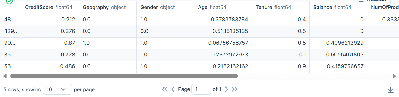
bank_df.head()
범주형, 정수형 및 부동 소수점 열이 있습니다. 데이터 세트는 꽤 깨끗해 보입니다.

간단한 Scikit-learn 코드
데이터 과학자로서 저는 이 코드를 여러 번 작성했습니다. 우리의 목표는 범주형 특성과 숫자 특성 모두에 대한 누락된 값을 채우는 것입니다. 이를 달성하기 위해 각 기능 유형에 대해 서로 다른 전략을 갖춘 `SimpleImputer`를 사용합니다.
누락된 값이 채워진 후 범주형 기능을 정수로 변환하고 숫자 기능에 최소-최대 스케일링을 적용합니다.
from sklearn.impute import SimpleImputer
from sklearn.preprocessing import OrdinalEncoder, MinMaxScaler

cat_col = [1,2]
num_col = [0,3,4,5,6,7,8,9]

# Filling missing categorical values
cat_impute = SimpleImputer(strategy="most_frequent")
bank_df.iloc[:,cat_col] = cat_impute.fit_transform(bank_df.iloc[:,cat_col])

# Filling missing numerical values
num_impute = SimpleImputer(strategy="median")
bank_df.iloc[:,num_col] = num_impute.fit_transform(bank_df.iloc[:,num_col])


# Encode categorical features as an integer array.
cat_encode = OrdinalEncoder()
bank_df.iloc[:,cat_col] = cat_encode.fit_transform(bank_df.iloc[:,cat_col])


# Scaling numerical values.
scaler = MinMaxScaler()
bank_df.iloc[:,num_col] = scaler.fit_transform(bank_df.iloc[:,num_col])

bank_df.head()
결과적으로 우리는 정수 또는 부동 소수점 값만으로 깨끗하고 변환된 데이터 세트를 얻었습니다.
Scikit-learn 파이프라인 코드
`Pipeline`과 `ColumnTransformer`를 사용하여 위 코드를 변환해 보겠습니다. 전처리 기술을 적용하는 대신 두 개의 파이프라인을 생성하겠습니다. 하나는 숫자 열용이고 다른 하나는 범주형 열용입니다.
- 수치 파이프라인에서 우리는 "평균" 전략으로 간단한 대체를 사용하고 정규화를 위해 최소-최대 스케일러를 적용했습니다.
- 범주형 파이프라인에서는 "most_frequent" 전략을 사용하는 단순 입력기와 원래 인코더를 사용하여 범주를 숫자 값으로 변환했습니다.
ColumnTransformer를 사용하여 두 파이프라인을 결합하고 각각에 열 인덱스를 제공했습니다. 특정 열에 이러한 파이프라인을 적용하는 데 도움이 됩니다. 예를 들어 범주형 변환기 파이프라인은 열 1과 2에만 적용됩니다.
참고 : 나머지=”통과”는 처리되지 않은 열이 결국 추가된다는 의미입니다. 우리의 경우에는 대상 열입니다.
from sklearn.impute import SimpleImputer
from sklearn.preprocessing import OrdinalEncoder, MinMaxScaler
from sklearn.compose import ColumnTransformer
from sklearn.pipeline import Pipeline


# Identify numerical and categorical columns
cat_col = [1,2]
num_col = [0,3,4,5,6,7,8,9]

# Transformers for numerical data
numerical_transformer = Pipeline(steps=[
    ('imputer', SimpleImputer(strategy='mean')),
    ('scaler', MinMaxScaler())
])

# Transformers for categorical data
categorical_transformer = Pipeline(steps=[
    ('imputer', SimpleImputer(strategy='most_frequent')),
    ('encoder', OrdinalEncoder())
])

# Combine transformers into a ColumnTransformer
preproc_pipe = ColumnTransformer(
    transformers=[
        ('num', numerical_transformer, num_col),
        ('cat', categorical_transformer, cat_col)
    ],
    remainder="passthrough"
)

# Apply the preprocessing pipeline
bank_df = preproc_pipe.fit_transform(bank_df)
bank_df[0]
변환 후 결과 배열에는 열 변환기의 파이프라인 순서에 따라 시작 부분의 숫자 변환 값과 끝 부분의 범주형 변환 값이 포함됩니다.
array([0.712     , 0.24324324, 0.6       , 0.        , 0.33333333,
       1.        , 1.        , 0.76443485, 2.        , 0.        ,
       0.        ])
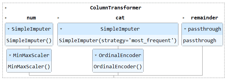
Jupyter Notebook에서 파이프라인 개체를 실행하여 파이프라인을 시각화할 수 있습니다. 최신 버전의 Scikit-learn이 있는지 확인하세요.
preproc_pipe
모델을 훈련하고 평가하려면 데이터 세트를 훈련과 테스트라는 두 가지 하위 집합으로 분할해야 합니다.
이를 위해 먼저 종속 변수와 독립 변수를 생성하고 이를 NumPy 배열로 변환합니다. 그런 다음 `train_test_split` 함수를 사용하여 데이터세트를 두 개의 하위 집합으로 분할합니다.
from sklearn.model_selection import train_test_split

X = bank_df.drop("Exited", axis=1).values
y = bank_df.Exited.values

X_train, X_test, y_train, y_test = train_test_split(
    X, y, test_size=0.3, random_state=125
)
간단한 Scikit-learn 코드
학습 코드를 작성하는 기존 방법은 먼저 'SelectKBest'를 사용하여 기능 선택을 수행한 다음 Random Forest Classifier 모델에 새로운 기능을 제공하는 것입니다.
먼저 훈련 세트를 사용하여 모델을 훈련하고 테스트 데이터 세트를 사용하여 결과를 평가합니다.
from sklearn.feature_selection import SelectKBest, chi2
from sklearn.ensemble import RandomForestClassifier

KBest = SelectKBest(chi2, k="all")
X_train = KBest.fit_transform(X_train, y_train)
X_test = KBest.transform(X_test)

model = RandomForestClassifier(n_estimators=100, random_state=125)

model.fit(X_train,y_train)

model.score(X_test, y_test)
우리는 상당히 좋은 정확도 점수를 얻었습니다.
0.8613035487063481Scikit-learn 파이프라인 코드
'파이프라인' 기능을 사용하여 두 학습 단계를 하나의 파이프라인으로 결합해 보겠습니다. 그런 다음 훈련 세트에 모델을 맞추고 테스트 세트에서 평가할 수 있습니다.
KBest = SelectKBest(chi2, k="all")
model = RandomForestClassifier(n_estimators=100, random_state=125)

train_pipe = Pipeline(
    steps=[
        ("KBest", KBest),
        ("RFmodel", model),
    ]
)

train_pipe.fit(X_train,y_train)

train_pipe.score(X_test, y_test)
비슷한 결과를 얻었지만 코드가 더 효율적이고 간단해 보입니다. 학습 파이프라인에서 새 단계를 추가하거나 제거하는 것은 매우 쉽습니다.
0.8613035487063481
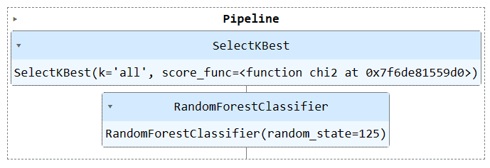
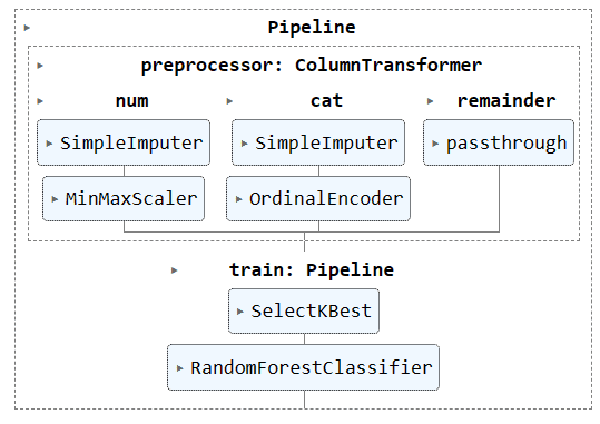
파이프라인 개체를 실행하여 파이프라인을 시각화합니다.
train_pipe
이제 다른 파이프라인을 생성하고 두 파이프라인을 모두 추가하여 전처리 파이프라인과 학습 파이프라인을 결합하겠습니다.
전체 코드는 다음과 같습니다.
import pandas as pd
from sklearn.model_selection import train_test_split
from sklearn.impute import SimpleImputer
from sklearn.preprocessing import OrdinalEncoder, MinMaxScaler
from sklearn.compose import ColumnTransformer
from sklearn.pipeline import Pipeline
from sklearn.feature_selection import SelectKBest, chi2
from sklearn.ensemble import RandomForestClassifier

#loading the data
bank_df = pd.read_csv("train.csv", index_col="id")
bank_df = bank_df.drop(['CustomerId', 'Surname'], axis=1)
bank_df = bank_df.sample(frac=1)


# Splitting data into training and testing sets
X = bank_df.drop(["Exited"],axis=1)
y = bank_df.Exited

X_train, X_test, y_train, y_test = train_test_split(
    X, y, test_size=0.3, random_state=125
)

# Identify numerical and categorical columns
cat_col = [1,2]
num_col = [0,3,4,5,6,7,8,9]

# Transformers for numerical data
numerical_transformer = Pipeline(steps=[
    ('imputer', SimpleImputer(strategy='mean')),
    ('scaler', MinMaxScaler())
])

# Transformers for categorical data
categorical_transformer = Pipeline(steps=[
    ('imputer', SimpleImputer(strategy='most_frequent')),
    ('encoder', OrdinalEncoder())
])

# Combine pipelines using ColumnTransformer
preproc_pipe = ColumnTransformer(
    transformers=[
        ('num', numerical_transformer, num_col),
        ('cat', categorical_transformer, cat_col)
    ],
    remainder="passthrough"
)

# Selecting the best features
KBest = SelectKBest(chi2, k="all")

# Random Forest Classifier
model = RandomForestClassifier(n_estimators=100, random_state=125)

# KBest and model pipeline
train_pipe = Pipeline(
    steps=[
        ("KBest", KBest),
        ("RFmodel", model),
    ]
)

# Combining the preprocessing and training pipelines
complete_pipe = Pipeline(
    steps=[

        ("preprocessor", preproc_pipe),
        ("train", train_pipe),
    ]
)

# running the complete pipeline
complete_pipe.fit(X_train,y_train)

# model accuracy
complete_pipe.score(X_test, y_test)
출력:
0.8592837955201874
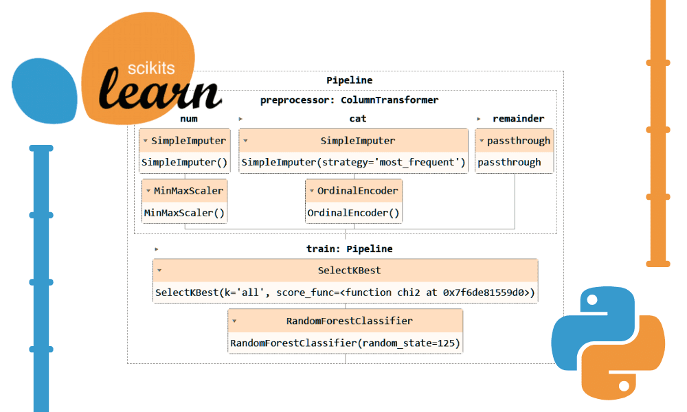
전체 파이프라인 시각화.
complete_pipe
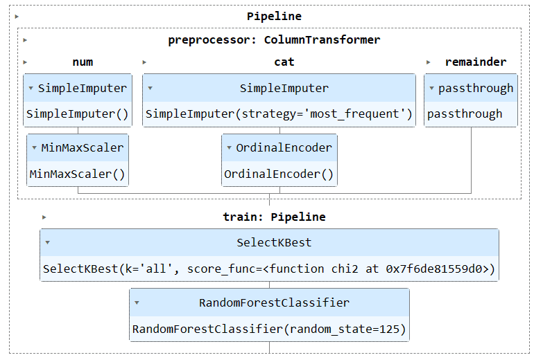
파이프라인 사용의 주요 이점 중 하나는 모델과 함께 파이프라인을 저장할 수 있다는 것입니다. 추론 중에는 원시 데이터를 처리하고 정확한 예측을 제공할 준비가 된 파이프라인 개체만 로드하면 됩니다. 앱 파일의 처리 및 변환 기능은 기본적으로 작동하므로 다시 작성할 필요가 없습니다. 이를 통해 기계 학습 워크플로가 더욱 효율적이고 시간이 절약됩니다.
먼저 다음을 사용하여 파이프라인을 저장해 보겠습니다. 스코프-개발/스코프 도서관.
import skops.io as sio

sio.dump(complete_pipe, "bank_pipeline.skops")
그런 다음 저장된 파이프라인을 로드하고 파이프라인을 표시합니다.
new_pipe = sio.load("bank_pipeline.skops", trusted=True)
new_pipe
보시다시피 파이프라인을 성공적으로 로드했습니다.
로드된 파이프라인을 평가하기 위해 테스트 세트에 대한 예측을 수행한 다음 정확도와 F1 점수를 계산합니다.
from sklearn.metrics import accuracy_score, f1_score

predictions = new_pipe.predict(X_test)
accuracy = accuracy_score(y_test, predictions)
f1 = f1_score(y_test, predictions, average="macro")

print("Accuracy:", str(round(accuracy, 2) * 100) + "%", "F1:", round(f1, 2))
f1 점수를 높이려면 소수 클래스에 집중해야 한다는 것이 밝혀졌습니다.
Accuracy: 86.0% F1: 0.76
프로젝트 파일과 코드는 다음에서 사용할 수 있습니다. 딥노트 작업공간. 작업공간에는 두 개의 노트북이 있습니다. 하나는 Scikit-learn 파이프라인이 있고 다른 하나는 Scikit-learn 파이프라인이 없습니다.
이 튜토리얼에서는 Scikit-learn 파이프라인이 데이터 변환 및 모델의 시퀀스를 함께 연결하여 기계 학습 워크플로를 간소화하는 데 어떻게 도움이 되는지 배웠습니다. 전처리와 모델 교육을 단일 파이프라인 개체에 결합함으로써 코드를 단순화하고 일관된 데이터 변환을 보장하며 워크플로를 보다 체계적이고 재현 가능하게 만들 수 있습니다.
아비드 알리 아완 (@1abidaliawan)은 기계 학습 모델 구축을 좋아하는 공인 데이터 과학자 전문가입니다. 현재 그는 콘텐츠 제작에 집중하고 있으며 머신 러닝 및 데이터 과학 기술에 대한 기술 블로그를 작성하고 있습니다. Abid는 기술 관리 석사 학위와 통신 공학 학사 학위를 보유하고 있습니다. 그의 비전은 정신 질환으로 고생하는 학생들을 위해 그래프 신경망을 사용하여 AI 제품을 만드는 것입니다.
- SEO 기반 콘텐츠 및 PR 배포. 오늘 증폭하십시오.
- PlatoData.Network 수직 생성 Ai. 자신에게 권한을 부여하십시오. 여기에서 액세스하십시오.
- PlatoAiStream. 웹3 인텔리전스. 지식 증폭. 여기에서 액세스하십시오.
- 플라톤ESG. 탄소, 클린테크, 에너지, 환경, 태양광, 폐기물 관리. 여기에서 액세스하십시오.
- PlatoHealth. 생명 공학 및 임상 시험 인텔리전스. 여기에서 액세스하십시오.
- 출처: https://www.kdnuggets.com/streamline-your-machine-learning-workflow-with-scikit-learn-pipelines?utm_source=rss&utm_medium=rss&utm_campaign=streamline-your-machine-learning-workflow-with-scikit-learn-pipelines

