Finite element methods for analysis crop up in many domains in electronic system design: mechanical stress analysis in multi-die systems, thermal analysis as a counterpart to both cooling and stress analysis (eg warping) and electromagnetic compliance analysis. (Computational fluid dynamics – CFD – is a different beast which I might cover in a separate blog.) I have covered topics in this area with another client and continue to find the domain attractive because it resonates with my physics background and my inner math geek (solving differential equations). Here I explore a recent paper from Siemens AG together with the Technical Universities of Munich and Braunschweig.

The problem statement

Finite element methods are techniques to numerically solve systems of 2D/3D partial differential equations (PDEs) arising in many physical analyses. These can extend from how heat diffuses in a complex SoC, to EM analyses for automotive radar, to how a mechanical structure bends under stress, to how the front of a car crumples in a crash.

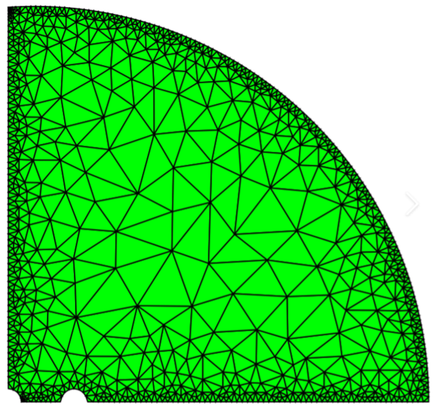
For FEM, a mesh is constructed across the physical space as a discrete framework for analysis, finer grained around boundaries and especially rapidly varying boundary conditions, and more coarse-grained elsewhere. Skipping the gory details, the method optimizes linear superpositions of simple functions across the mesh by varying coefficients in the superposition. Optimization aims to find a best fit within some acceptable tolerance consistent with discrete proxies for the PDEs together with initial conditions and boundary conditions through linear algebra and other methods.

Very large meshes are commonly needed to meet acceptable accuracy leading to very long run times for FEM solutions on realistic problems, becoming even more onerous when running multiple analyses to explore optimization possibilities. Each run essentially starts from scratch with no learning leverage between runs, which suggests an opportunity to use ML methods to accelerate analysis.

Ways to use ML with FEM

A widely used approach to accelerate FEM analyses (FEAs) is to build surrogate models. These are like abstract models in other domains – simplified versions of the full complexity of the original model. FEA experts talk about Reduced Order Models (ROMs) which continue to exhibit a good approximation of the (discretized) physical behavior of the source model but bypass the need to run FEA, at least in the design optimization phase,  though running much faster than FEA.

One way to build a surrogate would be to start with a bunch of FEAs, using that information as a training database to build the surrogate. However, this still requires lengthy analyses to generate training sets of inputs and outputs. The authors also point out another weakness in such an approach. ML has no native understanding of the physics constraints important in all such applications and is therefore prone to hallucination if presented with a scenario outside its training set.

Conversely, replacing FEM with a physically informed neural network (PINN) incorporates physical PDEs into loss function calculations, in essence introducing physical constraints into gradient-based optimizations. This is a clever idea though subsequent research has shown that while the method works on simple problems, it breaks down in the presence of high frequency and multi-scale features. Also disappointing is that the training time for such methods can be longer than FEA runtimes.

This paper suggests an intriguing alternative, to combine FEA and ML training more closely so that ML loss-functions train on the FEA error calculations in fitting trial solutions across the mesh. There is some similarity with the PINN approach but with an important difference: this neural net runs together with FEA to accelerate convergence to a solution in training. Which apparently results in faster training. In inference the neural net model runs without need for the FEA. By construction, a model trained in this way should conform closely to the physical constraints of the real problem since it has been trained very closely against a physically aware solver.

I think my interpretation here is fairly accurate. I welcome corrections from experts!

Share this post via:

• SEO Powered Content & PR Distribution. Get Amplified Today.
• PlatoData.Network Vertical Generative Ai. Empower Yourself. Access Here.
• PlatoAiStream. Web3 Intelligence. Knowledge Amplified. Access Here.
• PlatoESG. Carbon, CleanTech, Energy, Environment, Solar, Waste Management. Access Here.
• PlatoHealth. Biotech and Clinical Trials Intelligence. Access Here.
• Source: https://semiwiki.com/artificial-intelligence/341034-blending-finite-element-methods-and-ml/