著者による画像
Scikit-learn パイプラインを使用すると、前処理とモデリングの手順が簡素化され、コードの複雑さが軽減され、データ前処理の一貫性が確保され、ハイパーパラメータの調整が容易になり、ワークフローがより組織化されて保守しやすくなります。複数の変換と最終モデルを 1 つのエンティティに統合することで、パイプラインは再現性を高め、すべてをより効率的にします。
このチュートリアルでは、 銀行チャーン ランダム フォレスト分類器をトレーニングするための Kaggle のデータセット。データ前処理とモデル トレーニングの従来のアプローチと、Scikit-learn パイプラインと ColumnTransformers を使用したより効率的な方法を比較します。
データ処理パイプラインでは、カテゴリ列と数値列の両方を個別に変換する方法を学びます。従来のスタイルのコードから始めて、同様の処理を実行するより良い方法を示します。
zip ファイルからデータを抽出した後、「id」をインデックス列として指定した `train.csv` ファイルをロードします。不要な列を削除し、データセットをシャッフルします。
import pandas as pd
bank_df = pd.read_csv("train.csv", index_col="id")
bank_df = bank_df.drop(['CustomerId', 'Surname'], axis=1)
bank_df = bank_df.sample(frac=1)
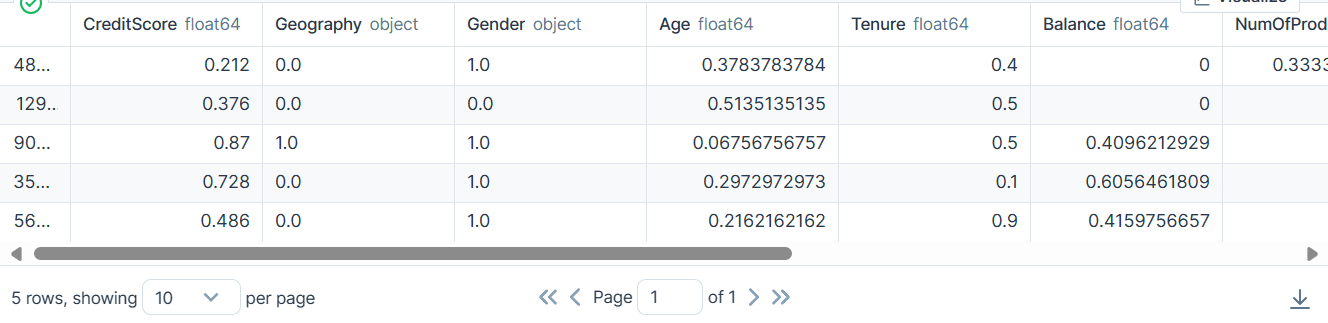
bank_df.head()
カテゴリ列、整数列、および浮動小数点列があります。データセットはかなりきれいに見えます。

単純な Scikit-Learn コード
データ サイエンティストとして、私はこのコードを何度も作成しました。私たちの目的は、カテゴリ特徴と数値特徴の両方の欠損値を埋めることです。これを実現するために、機能の種類ごとに異なる戦略を持つ `SimpleImputer` を使用します。
欠損値が埋められた後、カテゴリ特徴を整数に変換し、数値特徴に最小-最大スケーリングを適用します。
from sklearn.impute import SimpleImputer
from sklearn.preprocessing import OrdinalEncoder, MinMaxScaler

cat_col = [1,2]
num_col = [0,3,4,5,6,7,8,9]

# Filling missing categorical values
cat_impute = SimpleImputer(strategy="most_frequent")
bank_df.iloc[:,cat_col] = cat_impute.fit_transform(bank_df.iloc[:,cat_col])

# Filling missing numerical values
num_impute = SimpleImputer(strategy="median")
bank_df.iloc[:,num_col] = num_impute.fit_transform(bank_df.iloc[:,num_col])


# Encode categorical features as an integer array.
cat_encode = OrdinalEncoder()
bank_df.iloc[:,cat_col] = cat_encode.fit_transform(bank_df.iloc[:,cat_col])


# Scaling numerical values.
scaler = MinMaxScaler()
bank_df.iloc[:,num_col] = scaler.fit_transform(bank_df.iloc[:,num_col])

bank_df.head()
その結果、整数値または浮動小数点値のみを使用して変換されたクリーンなデータセットが得られました。
Scikit-learn パイプライン コード
上記のコードを`Pipeline`と`ColumnTransformer`を使って変換してみましょう。前処理手法を適用する代わりに、2 つのパイプラインを作成します。 1 つは数値列用で、もう 1 つはカテゴリ列用です。
- 数値パイプラインでは、「平均」戦略による単純な代入を使用し、正規化のために最小-最大スケーラーを適用しました。
- カテゴリ パイプラインでは、「most_frequent」戦略を備えた単純なインピューターとオリジナルのエンコーダーを使用して、カテゴリを数値に変換しました。
ColumnTransformer を使用して 1 つのパイプラインを結合し、それぞれに列インデックスを提供しました。これは、これらのパイプラインを特定の列に適用するのに役立ちます。たとえば、カテゴリカル変換パイプラインは列 2 と列 XNUMX にのみ適用されます。
注: 残り =”パススルー” は、処理されていない列が最後に追加されることを意味します。この例では、それがターゲット列です。
from sklearn.impute import SimpleImputer
from sklearn.preprocessing import OrdinalEncoder, MinMaxScaler
from sklearn.compose import ColumnTransformer
from sklearn.pipeline import Pipeline


# Identify numerical and categorical columns
cat_col = [1,2]
num_col = [0,3,4,5,6,7,8,9]

# Transformers for numerical data
numerical_transformer = Pipeline(steps=[
    ('imputer', SimpleImputer(strategy='mean')),
    ('scaler', MinMaxScaler())
])

# Transformers for categorical data
categorical_transformer = Pipeline(steps=[
    ('imputer', SimpleImputer(strategy='most_frequent')),
    ('encoder', OrdinalEncoder())
])

# Combine transformers into a ColumnTransformer
preproc_pipe = ColumnTransformer(
    transformers=[
        ('num', numerical_transformer, num_col),
        ('cat', categorical_transformer, cat_col)
    ],
    remainder="passthrough"
)

# Apply the preprocessing pipeline
bank_df = preproc_pipe.fit_transform(bank_df)
bank_df[0]
変換後の結果の配列には、列トランスフォーマー内のパイプラインの順序に基づいて、開始時に数値変換値が含まれ、最後にカテゴリカル変換値が含まれます。
array([0.712     , 0.24324324, 0.6       , 0.        , 0.33333333,
       1.        , 1.        , 0.76443485, 2.        , 0.        ,
       0.        ])
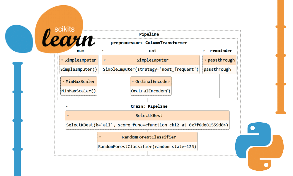
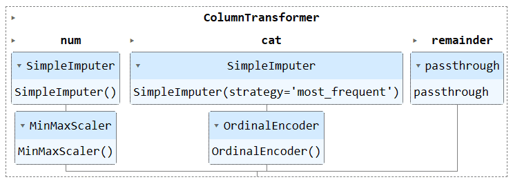
Jupyter Notebook でパイプライン オブジェクトを実行して、パイプラインを視覚化できます。 Scikit-learn の最新バージョンを使用していることを確認してください。
preproc_pipe
モデルをトレーニングして評価するには、データセットをトレーニングとテストの 2 つのサブセットに分割する必要があります。
これを行うには、まず従属変数と独立変数を作成し、それらを NumPy 配列に変換します。次に、`train_test_split` 関数を使用して、データセットを 2 つのサブセットに分割します。
from sklearn.model_selection import train_test_split

X = bank_df.drop("Exited", axis=1).values
y = bank_df.Exited.values

X_train, X_test, y_train, y_test = train_test_split(
    X, y, test_size=0.3, random_state=125
)
単純な Scikit-Learn コード
トレーニング コードを記述する従来の方法は、最初に「SelectKBest」を使用して特徴選択を実行し、次に新しい特徴をランダム フォレスト分類子モデルに提供することです。
まずトレーニング セットを使用してモデルをトレーニングし、テスト データセットを使用して結果を評価します。
from sklearn.feature_selection import SelectKBest, chi2
from sklearn.ensemble import RandomForestClassifier

KBest = SelectKBest(chi2, k="all")
X_train = KBest.fit_transform(X_train, y_train)
X_test = KBest.transform(X_test)

model = RandomForestClassifier(n_estimators=100, random_state=125)

model.fit(X_train,y_train)

model.score(X_test, y_test)
かなり良い精度スコアを達成しました。
0.8613035487063481Scikit-learn パイプライン コード
「Pipeline」関数を使用して、両方のトレーニング ステップをパイプラインに結合してみましょう。その後、モデルをトレーニング セットに適合させ、テスト セットで評価できます。
KBest = SelectKBest(chi2, k="all")
model = RandomForestClassifier(n_estimators=100, random_state=125)

train_pipe = Pipeline(
    steps=[
        ("KBest", KBest),
        ("RFmodel", model),
    ]
)

train_pipe.fit(X_train,y_train)

train_pipe.score(X_test, y_test)
同様の結果が得られましたが、コードはより効率的で簡単になっているようです。トレーニング パイプラインに新しいステップを追加または削除するのは非常に簡単です。
0.8613035487063481
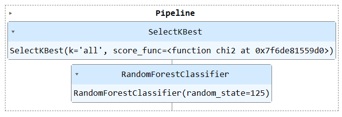
パイプライン オブジェクトを実行してパイプラインを視覚化します。
train_pipe
次に、別のパイプラインを作成し、両方のパイプラインを追加することで、前処理パイプラインとトレーニング パイプラインの両方を結合します。
完全なコードは次のとおりです。
import pandas as pd
from sklearn.model_selection import train_test_split
from sklearn.impute import SimpleImputer
from sklearn.preprocessing import OrdinalEncoder, MinMaxScaler
from sklearn.compose import ColumnTransformer
from sklearn.pipeline import Pipeline
from sklearn.feature_selection import SelectKBest, chi2
from sklearn.ensemble import RandomForestClassifier

#loading the data
bank_df = pd.read_csv("train.csv", index_col="id")
bank_df = bank_df.drop(['CustomerId', 'Surname'], axis=1)
bank_df = bank_df.sample(frac=1)


# Splitting data into training and testing sets
X = bank_df.drop(["Exited"],axis=1)
y = bank_df.Exited

X_train, X_test, y_train, y_test = train_test_split(
    X, y, test_size=0.3, random_state=125
)

# Identify numerical and categorical columns
cat_col = [1,2]
num_col = [0,3,4,5,6,7,8,9]

# Transformers for numerical data
numerical_transformer = Pipeline(steps=[
    ('imputer', SimpleImputer(strategy='mean')),
    ('scaler', MinMaxScaler())
])

# Transformers for categorical data
categorical_transformer = Pipeline(steps=[
    ('imputer', SimpleImputer(strategy='most_frequent')),
    ('encoder', OrdinalEncoder())
])

# Combine pipelines using ColumnTransformer
preproc_pipe = ColumnTransformer(
    transformers=[
        ('num', numerical_transformer, num_col),
        ('cat', categorical_transformer, cat_col)
    ],
    remainder="passthrough"
)

# Selecting the best features
KBest = SelectKBest(chi2, k="all")

# Random Forest Classifier
model = RandomForestClassifier(n_estimators=100, random_state=125)

# KBest and model pipeline
train_pipe = Pipeline(
    steps=[
        ("KBest", KBest),
        ("RFmodel", model),
    ]
)

# Combining the preprocessing and training pipelines
complete_pipe = Pipeline(
    steps=[

        ("preprocessor", preproc_pipe),
        ("train", train_pipe),
    ]
)

# running the complete pipeline
complete_pipe.fit(X_train,y_train)

# model accuracy
complete_pipe.score(X_test, y_test)
出力:
0.8592837955201874
完全なパイプラインを視覚化します。
complete_pipe
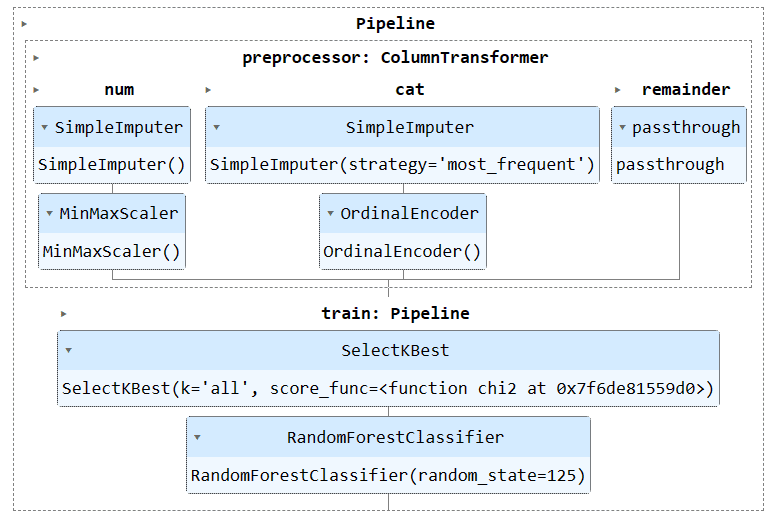
パイプラインを使用する主な利点の 1 つは、モデルと一緒にパイプラインを保存できることです。推論中は、パイプライン オブジェクトを読み込むだけで、すぐに生データを処理して正確な予測が提供されます。すぐに機能するため、アプリ ファイル内の処理関数と変換関数を書き直す必要はありません。これにより、機械学習のワークフローがより効率的になり、時間が節約されます。
まず、次のコマンドを使用してパイプラインを保存しましょう。 skops-dev/skops としょうかん。
import skops.io as sio

sio.dump(complete_pipe, "bank_pipeline.skops")
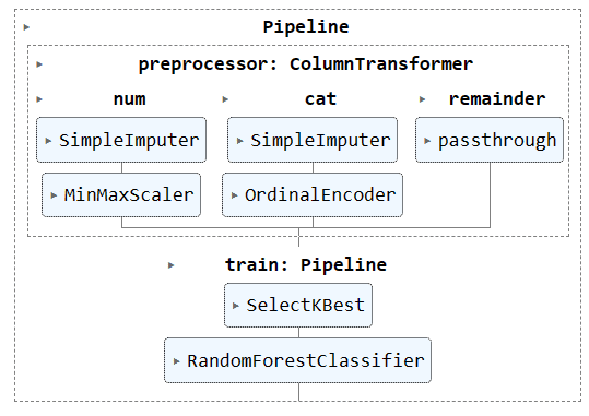
次に、保存したパイプラインをロードし、パイプラインを表示します。
new_pipe = sio.load("bank_pipeline.skops", trusted=True)
new_pipe
ご覧のとおり、パイプラインが正常にロードされました。
読み込まれたパイプラインを評価するために、テスト セットで予測を行い、精度と F1 スコアを計算します。
from sklearn.metrics import accuracy_score, f1_score

predictions = new_pipe.predict(X_test)
accuracy = accuracy_score(y_test, predictions)
f1 = f1_score(y_test, predictions, average="macro")

print("Accuracy:", str(round(accuracy, 2) * 100) + "%", "F1:", round(f1, 2))
f1スコアを向上させるには、少数民族に焦点を当てる必要があることがわかりました。
Accuracy: 86.0% F1: 0.76
プロジェクト ファイルとコードは次の場所で入手できます。 ディープノートワークスペース。ワークスペースには 2 つのノートブックがあります。1 つは Scikit-learn パイプラインを備えており、もう 1 つはそれを備えていません。
このチュートリアルでは、Scikit-learn パイプラインがデータ変換とモデルのシーケンスを連結することで機械学習ワークフローの合理化にどのように役立つかを学びました。前処理とモデル トレーニングを単一の Pipeline オブジェクトに組み合わせることで、コードを簡素化し、一貫したデータ変換を確保し、ワークフローをより組織化して再現可能にすることができます。
アビッド・アリ・アワン (@ 1abidaliawan)は、機械学習モデルの構築を愛する認定データサイエンティストの専門家です。 現在、彼はコンテンツの作成と、機械学習とデータサイエンステクノロジーに関する技術ブログの執筆に注力しています。 Abidは、技術管理の修士号と電気通信工学の学士号を取得しています。 彼のビジョンは、精神疾患に苦しんでいる学生のためにグラフニューラルネットワークを使用してAI製品を構築することです。
- SEO を活用したコンテンツと PR 配信。 今日増幅されます。
- PlatoData.Network 垂直生成 Ai。 自分自身に力を与えましょう。 こちらからアクセスしてください。
- プラトアイストリーム。 Web3 インテリジェンス。 知識増幅。 こちらからアクセスしてください。
- プラトンESG。 カーボン、 クリーンテック、 エネルギー、 環境、 太陽、 廃棄物管理。 こちらからアクセスしてください。
- プラトンヘルス。 バイオテクノロジーと臨床試験のインテリジェンス。 こちらからアクセスしてください。
- 情報源: https://www.kdnuggets.com/streamline-your-machine-learning-workflow-with-scikit-learn-pipelines?utm_source=rss&utm_medium=rss&utm_campaign=streamline-your-machine-learning-workflow-with-scikit-learn-pipelines

