Introduction

In machine learning, the bias-variance trade-off is a fundamental concept affecting the performance of any predictive model. It refers to the delicate balance between bias error and variance error of a model, as it is impossible to simultaneously minimize both. Striking the right balance is crucial for achieving optimal model performance.

In this short article, we’ll define bias and variance, explain how they affect a machine learning model, and provide some practical advice on how to deal with them in practice.

Understanding Bias and Variance

Before diving into the relationship between bias and variance, let’s define what these terms represent in machine learning.

Bias error refers to the difference between the prediction of a model and the correct values it tries to predict (ground truth). In other words, bias is the error a model commits due to its incorrect assumptions about the underlying data distribution. High bias models are often too simplistic, failing to capture the complexity of the data, leading to underfitting.

Variance error, on the other hand, refers to the model’s sensitivity to small fluctuations in the training data. High variance models are overly complex and tend to fit the noise in the data, rather than the underlying pattern, leading to overfitting. This results in poor performance on new, unseen data.

High bias can lead to underfitting, where the model is too simple to capture the complexity of the data. It makes strong assumptions about the data and fails to capture the true relationship between input and output variables. On the other hand, high variance can lead to overfitting, where the model is too complex and learns the noise in the data rather than the underlying relationship between input and output variables. Thus, overfitting models tend to fit the training data too closely and will not generalize well to new data, while underfitting models are not even able to fit the training data accurately.

As mentioned earlier, bias and variance are related, and a good model balances between bias error and variance error. The bias-variance trade-off is the process of finding the optimal balance between these two sources of error. A model with low bias and low variance will likely perform well on both training and new data, minimizing the total error.

The Bias-Variance Trade-Off

Achieving a balance between model complexity and its ability to generalize to unknown data is the core of the bias-variance tradeoff. In general, a more complex model will have a lower bias but higher variance, while a simpler model will have a higher bias but lower variance.

Since it is impossible to simultaneously minimize bias and variance, finding the optimal balance between them is crucial in building a robust machine learning model. For example, as we increase the complexity of a model, we also increase the variance. This is because a more complex model is more likely to fit the noise in the training data, which will lead to overfitting.

On the other hand, if we keep the model too simple, we will increase the bias. This is because a simpler model will not be able to capture the underlying relationships in the data, which will lead to underfitting.

The goal is to train a model that is complex enough to capture the underlying relationships in the training data, but not so complex that it fits the noise in the training data.

Bias-Variance Trade-Off in Practice

To diagnose model performance, we typically calculate and compare the train and validation errors. A useful tool for visualizing this is a plot of the learning curves, which displays the performance of the model on both the train and validation data throughout the training process. By examining these curves, we can determine whether a model is overfitting (high variance), underfitting (high bias), or well-fitting (optimal balance between bias and variance).

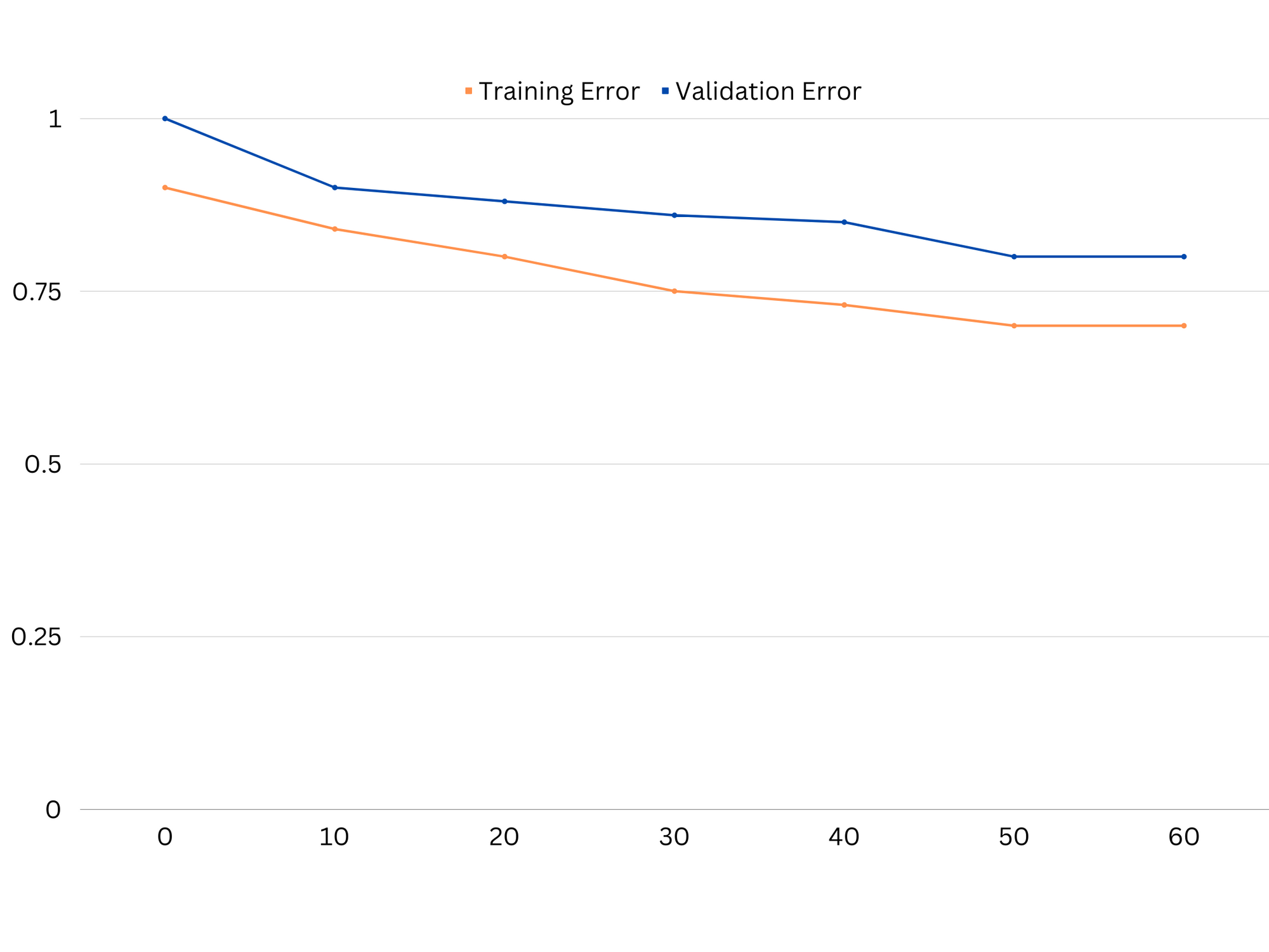
Example of learning curves of an underfitting model. Both train error and validation error are high.

In practice, low performance on both training and validation data suggests that the model is too simple, leading to underfitting. On the other hand, if the model performs very well on the training data but poorly on the test data, the model complexity is likely too high, resulting in overfitting. To address underfitting, we can try increasing the model complexity by adding more features, changing the learning algorithm, or choosing different hyperparameters. In the case of overfitting, we should consider regularizing the model or using techniques like cross-validation to improve its generalization capabilities.

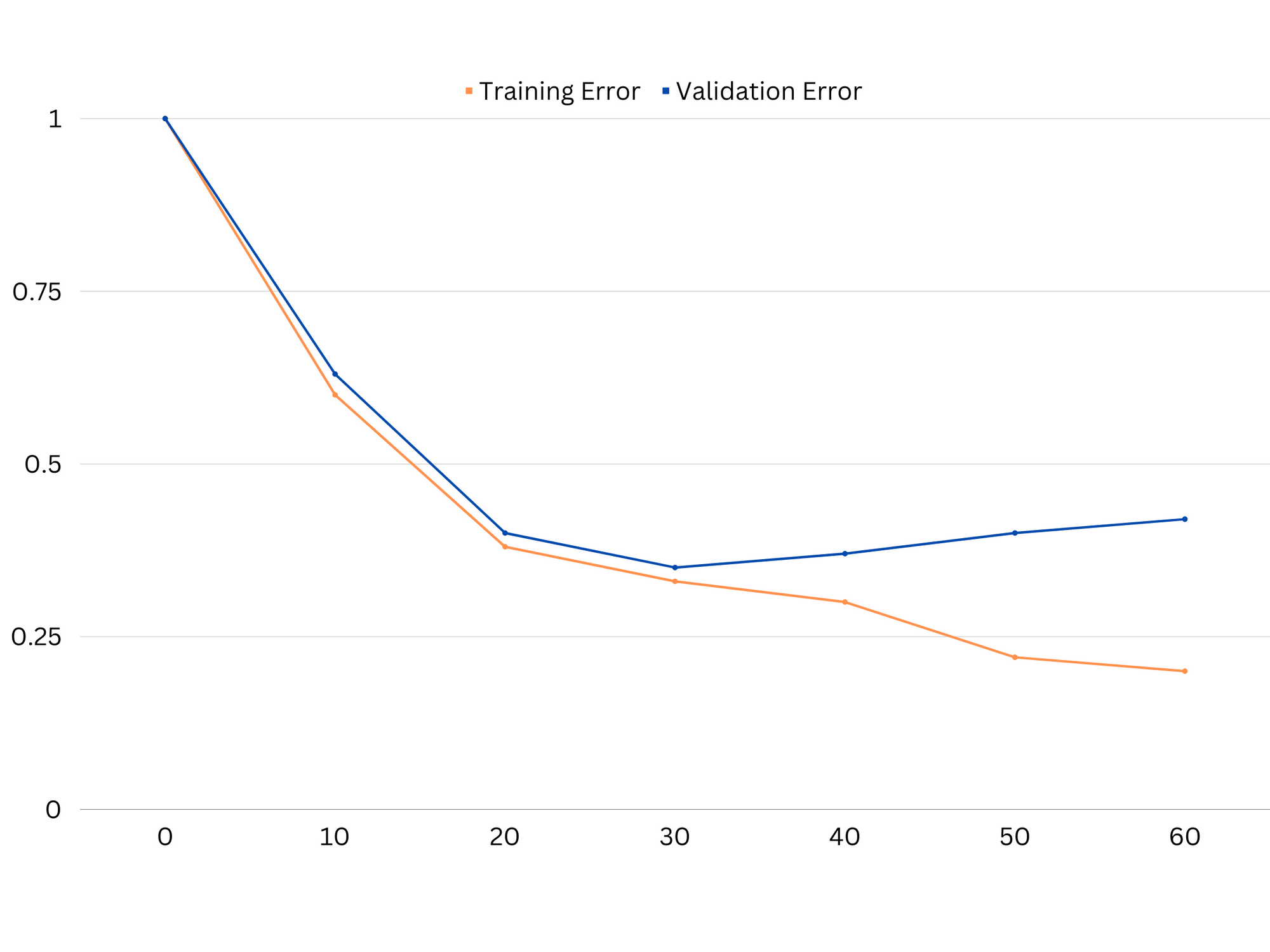
Example of learning curves of an overfitting model. Train error decreases while validation error begins to increase. The model is unable to generalize.

Regularization is a technique that can be used to reduce the variance error in machine learning models, helping to address the bias-variance trade-off. There are a number of different regularization techniques, each with their own advantages and disadvantages. Some popular regularization techniques include ridge regression, lasso regression, and elastic net regularization. All these techniques help prevent overfitting by adding a penalty term to the model’s objective function, which discourages extreme parameter values and encourages simpler models.

Ridge regression, also known as L2 regularization, adds a penalty term proportional to the square of the model parameters. This technique tends to result in models with smaller parameter values, which can lead to reduced variance and improved generalization. However, it does not perform feature selection, so all features remain in the model.

Lasso regression, or L1 regularization, adds a penalty term proportional to the absolute value of the model parameters. This technique can lead to models with sparse parameter values, effectively performing feature selection by setting some parameters to zero. This can result in simpler models that are easier to interpret.

Elastic net regularization is a combination of both L1 and L2 regularization, allowing for a balance between ridge and lasso regression. By controlling the ratio between the two penalty terms, elastic net can achieve the benefits of both techniques, such as improved generalization and feature selection.

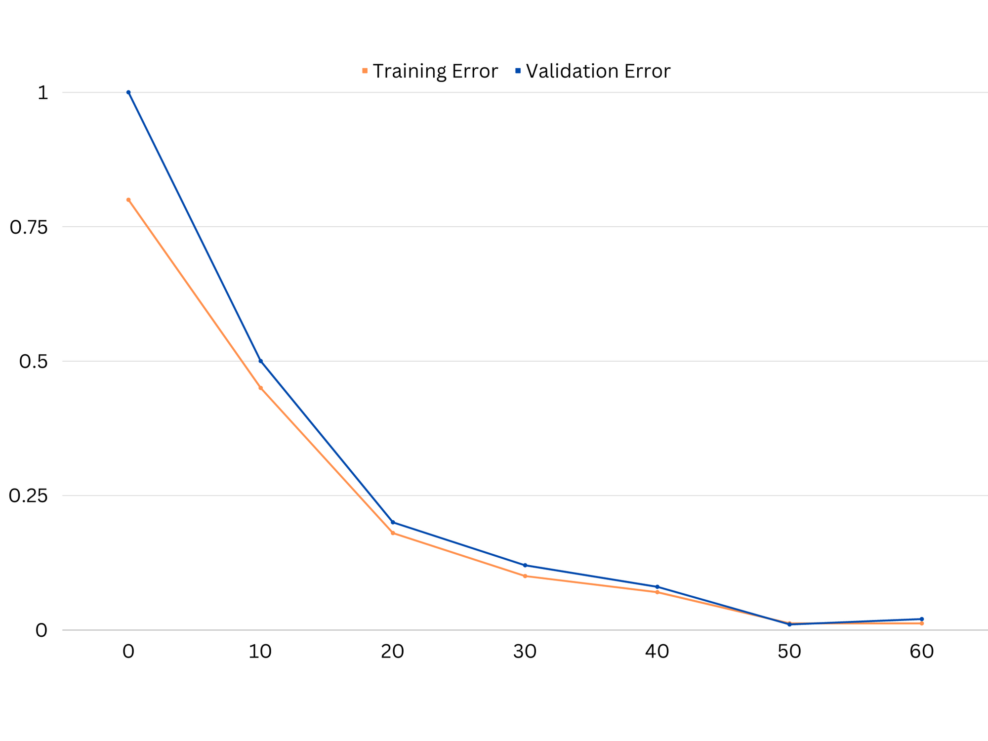
Example of learning curves of good fitting model.

Conclusions

The bias-variance trade-off is a crucial concept in machine learning that determines the effectiveness and goodness of a model. While high bias leads to underfitting and high variance leads to overfitting, finding the optimal balance between the two is necessary for building robust models that generalize well to new data.

With the help of learning curves, it is possible to identify overfitting or underfitting problems, and by tuning the complexity of the model or implementing regularization techniques, it is possible to improve the performance on both training and validation data, as well as test data.

• SEO Powered Content & PR Distribution. Get Amplified Today.
• PlatoAiStream. Web3 Data Intelligence. Knowledge Amplified. Access Here.
• Minting the Future w Adryenn Ashley. Access Here.
• Buy and Sell Shares in PRE-IPO Companies with PREIPO®. Access Here.
• Source: https://stackabuse.com/the-bias-variance-trade-off-in-machine-learning/