
개요
우리의 종합에 오신 것을 환영합니다 데이터 분석 Netflix의 세계를 깊이 파고드는 블로그. 전 세계 최고의 스트리밍 플랫폼 중 하나인 Netflix는 우리가 엔터테인먼트를 소비하는 방식을 혁신했습니다. 방대한 영화 및 TV 프로그램 라이브러리를 통해 전 세계 시청자에게 다양한 선택권을 제공합니다.
Netflix의 글로벌 도달 범위
Netflix는 놀라운 성장을 경험했으며 스트리밍 산업에서 지배적인 세력이 되기 위해 입지를 확장했습니다. 다음은 글로벌 영향을 보여주는 몇 가지 주목할만한 통계입니다.
- 사용자 기반: 2022년 XNUMX분기 초까지 Netflix는 약 222억 XNUMX만 명의 해외 가입자, 190개 이상의 국가(중국, 크림, 북한, 러시아 및 시리아 제외)에 걸쳐 있습니다. 이러한 인상적인 수치는 전 세계 시청자 사이에서 플랫폼의 광범위한 수용과 인기를 강조합니다.
- 국제적 확장: 190개 이상의 국가에서 사용할 수 있는 Netflix는 성공적으로 글로벌 입지를 구축했습니다. 회사는 다양한 언어로 자막과 더빙을 제공하여 다양한 청중에게 접근성을 보장함으로써 콘텐츠를 현지화하기 위해 상당한 노력을 기울였습니다.
이 블로그에서는 Netflix의 콘텐츠 환경에 숨겨진 흥미로운 패턴, 트렌드 및 통찰력을 탐구하는 흥미진진한 여정을 시작합니다. 의 힘을 활용 Python 및 그 데이터 분석 라이브러리에서 콘텐츠 추가, 재생 시간 분포, 장르 상관 관계, 제목과 설명에서 가장 일반적으로 사용되는 단어까지 밝혀주는 귀중한 정보를 발견하기 위해 방대한 Netflix 제품 컬렉션을 자세히 살펴봅니다.
자세한 코드 스니펫과 시각화, 플랫폼이 어떻게 진화했는지에 대한 새로운 관점을 제공하기 위해 Netflix의 콘텐츠 생태계 계층을 벗겨냅니다. 출시 패턴, 계절별 추세, 시청자 선호도를 분석하여 Netflix의 광대한 세계 내에서 콘텐츠의 역학 관계를 더 잘 이해하는 것을 목표로 합니다.
이 기사는 데이터 과학 Blogathon.
차례
데이터 준비
이 사례 연구에 사용된 데이터는 데이터 과학 및 기계 학습 애호가를 위한 인기 있는 플랫폼인 Kaggle에서 제공됩니다. "라는 제목의 데이터 세트Netflix 영화 및 TV 프로그램,”는 Kaggle에서 공개적으로 사용할 수 있으며 Netflix 스트리밍 플랫폼의 영화 및 TV 프로그램에 대한 귀중한 정보를 제공합니다.
데이터 세트는 각 영화 또는 TV 프로그램의 다양한 측면을 설명하는 다양한 열을 포함하는 표 형식으로 구성됩니다. 다음은 열과 해당 설명을 요약한 표입니다.
| 열 이름 | 상품 설명 |
|---|---|
| show_id | 모든 영화/TV 프로그램의 고유 ID |
| 유형 | 식별자 – 영화 또는 TV 프로그램 |
| 제목 | 영화/TV 프로그램 제목 |
| 이사 | 영화 감독 |
| 캐스트 | 영화 / 쇼에 참여하는 배우 |
| 국가 | 영화/쇼가 제작된 국가 |
| 날짜_추가됨 | Netflix에 추가된 날짜 |
| 출시년 | 영화/쇼의 실제 개봉 연도 |
| 평가 | 영화/쇼의 TV 등급 |
| 지속 | 총 기간 – 분 또는 시즌 수 |
이 섹션에서는 Netflix 데이터 세트에 대한 데이터 준비 작업을 수행하여 분석을 위한 청결성과 적합성을 보장합니다. 누락된 값과 중복을 처리하고 필요에 따라 데이터 유형 변환을 수행합니다. 코드를 살펴보고 각 단계를 살펴보겠습니다.
라이브러리 가져 오기
시작하려면 데이터 분석 및 시각화에 필요한 라이브러리를 가져옵니다. 이러한 라이브러리에는 다음이 포함됩니다. 팬더, numpy 및 matplotlib. pyplot 및 seaborn. 데이터를 효과적으로 조작하고 시각화하기 위한 필수 기능과 도구를 제공합니다.
# Importing necessary libraries for data analysis and visualization
import pandas as pd # pandas for data manipulation and analysis
import numpy as np # numpy for numerical operations
import matplotlib.pyplot as plt # matplotlib for data visualization
import seaborn as sns # seaborn for enhanced data visualization
데이터 세트 로드
다음으로 pd.read_csv() 함수를 사용하여 Netflix 데이터 세트를 로드합니다. 데이터 세트는 'netflix.csv' 파일에 저장됩니다. 구조를 이해하기 위해 데이터 세트의 처음 XNUMX개 레코드를 살펴보겠습니다.
# Loading the dataset from a CSV file
df = pd.read_csv('netflix.csv') # Displaying the first few rows of the dataset
df.head()
기술 통계
통해 데이터셋의 전반적인 특성을 이해하는 것이 중요합니다. 설명 통계. 개수, 평균, 표준 편차, 최소값, 최대값 및 사분위수와 같은 수치 속성에 대한 통찰력을 얻을 수 있습니다.
# Computing descriptive statistics for the dataset
df.describe()
간결한 요약
데이터 세트의 간결한 요약을 얻기 위해 df.info() 함수를 사용합니다. null이 아닌 값의 수와 각 열의 데이터 유형에 대한 정보를 제공합니다. 이 요약은 누락된 값과 데이터 유형의 잠재적인 문제를 식별하는 데 도움이 됩니다.
# Obtaining information about the dataset
df.info()
결 측값 처리
누락된 값은 정확한 분석을 방해할 수 있습니다. 이 데이터 세트는 df를 사용하여 각 열에서 누락된 값을 탐색합니다. isnull().sum(). 누락된 값이 있는 열을 식별하고 각 열에서 누락된 데이터의 백분율을 결정하는 것을 목표로 합니다.
# Checking for missing values in the dataset
df.isnull().sum()
누락된 값을 처리하기 위해 열마다 다른 전략을 사용합니다. 각 단계를 살펴보겠습니다.
중복
중복은 분석 결과를 왜곡할 수 있으므로 이를 해결하는 것이 필수적입니다. df.duplicated().sum()을 사용하여 중복 레코드를 식별하고 제거합니다.
# Checking for duplicate rows in the dataset
df.duplicated().sum()
특정 열의 누락된 값 처리
'디렉터' 및 '캐스트' 열의 경우 누락된 값을 '데이터 없음'으로 대체하여 데이터 무결성을 유지하고 분석의 편향을 방지합니다.
# Replacing missing values in the 'director' column with 'No Data'
df['director'].replace(np.nan, 'No Data', inplace=True) # Replacing missing values in the 'cast' column with 'No Data'
df['cast'].replace(np.nan, 'No Data', inplace=True)
'국가' 열에서 누락된 값을 모드(가장 자주 발생하는 값)로 채워 일관성을 유지하고 데이터 손실을 최소화합니다.
# Filling missing values in the 'country' column with the mode value
df['country'] = df['country'].fillna(df['country'].mode()[0])
'등급' 열의 경우 쇼의 '유형'에 따라 누락된 값을 채웁니다. 영화와 TV 프로그램에 대해 '등급' 모드를 별도로 지정합니다.
# Finding the mode rating for movies and TV shows
movie_rating = df.loc[df['type'] == 'Movie', 'rating'].mode()[0]
tv_rating = df.loc[df['type'] == 'TV Show', 'rating'].mode()[0] # Filling missing rating values based on the type of content
df['rating'] = df.apply(lambda x: movie_rating if x['type'] == 'Movie' and pd.isna(x['rating']) else tv_rating if x['type'] == 'TV Show' and pd.isna(x['rating']) else x['rating'], axis=1)
'기간' 열의 경우 쇼의 '유형'에 따라 누락된 값을 채웁니다. 영화와 TV 프로그램의 '기간' 모드를 별도로 지정합니다.
# Finding the mode duration for movies and TV shows
movie_duration_mode = df.loc[df['type'] == 'Movie', 'duration'].mode()[0]
tv_duration_mode = df.loc[df['type'] == 'TV Show', 'duration'].mode()[0] # Filling missing duration values based on the type of content
df['duration'] = df.apply(lambda x: movie_duration_mode if x['type'] == 'Movie' and pd.isna(x['duration']) else tv_duration_mode if x['type'] == 'TV Show' and pd.isna(x['duration']) else x['duration'], axis=1)
나머지 결측값 삭제
특정 열에서 누락된 값을 처리한 후 누락된 값이 있는 나머지 행을 모두 삭제하여 분석을 위한 깨끗한 데이터 세트를 보장합니다.
# Dropping rows with missing values
df.dropna(inplace=True)
날짜 처리
날짜 관련 속성을 기반으로 추가 분석이 가능하도록 pd.to_datetime()을 사용하여 'date_added' 열을 datetime 형식으로 변환합니다.
# Converting the 'date_added' column to datetime format
df["date_added"] = pd.to_datetime(df['date_added'])
추가 데이터 변환
'date_added' 열에서 추가 속성을 추출하여 분석 기능을 강화합니다. 이러한 시간적 측면을 기반으로 추세를 분석하기 위해 월 및 연도 값을 제거합니다.
# Extracting month, month name, and year from the 'date_added' column
df['month_added'] = df['date_added'].dt.month
df['month_name_added'] = df['date_added'].dt.month_name()
df['year_added'] = df['date_added'].dt.year
데이터 변환: 출연진, 국가, 출연진 및 감독
범주 속성을 보다 효과적으로 분석하기 위해 별도의 데이터 프레임으로 변환하여 보다 여유롭게 탐색하고 분석할 수 있습니다.
'cast', 'country', 'listed_in' 및 'director' 열의 경우 쉼표 구분 기호를 기준으로 값을 분할하고 각 값에 대해 별도의 행을 생성했습니다. 이러한 변환을 통해 보다 세분화된 수준에서 데이터를 분석할 수 있습니다.
# Splitting and expanding the 'cast' column
df_cast = df['cast'].str.split(',', expand=True).stack()
df_cast = df_cast.reset_index(level=1, drop=True).to_frame('cast')
df_cast['show_id'] = df['show_id'] # Splitting and expanding the 'country' column
df_country = df['country'].str.split(',', expand=True).stack()
df_country = df_country.reset_index(level=1, drop=True).to_frame('country')
df_country['show_id'] = df['show_id'] # Splitting and expanding the 'listed_in' column
df_listed_in = df['listed_in'].str.split(',', expand=True).stack()
df_listed_in = df_listed_in.reset_index(level=1, drop=True).to_frame('listed_in')
df_listed_in['show_id'] = df['show_id'] # Splitting and expanding the 'director' column
df_director = df['director'].str.split(',', expand=True).stack()
df_director = df_director.reset_index(level=1, drop=True).to_frame('director')
df_director['show_id'] = df['show_id']
이러한 데이터 준비 단계를 완료하면 추가 분석을 위해 깨끗하고 변환된 데이터 세트가 준비됩니다. 이러한 초기 데이터 조작은 Netflix 데이터 세트를 탐색하고 스트리밍 플랫폼의 데이터 기반 전략에 대한 통찰력을 발견하기 위한 기반을 설정합니다.
탐색 적 데이터 분석
콘텐츠 유형의 배포
Netflix 라이브러리의 콘텐츠 배포를 확인하기 위해 다음 코드를 사용하여 콘텐츠 유형(영화 및 TV 프로그램)의 배포 비율을 계산할 수 있습니다.
# Calculate the percentage distribution of content types
x = df.groupby(['type'])['type'].count()
y = len(df)
r = ((x/y) * 100).round(2) # Create a DataFrame to store the percentage distribution
mf_ratio = pd.DataFrame(r)
mf_ratio.rename({'type': '%'}, axis=1, inplace=True) # Plot the 3D-effect pie chart
plt.figure(figsize=(12, 8))
colors = ['#b20710', '#221f1f']
explode = (0.1, 0)
plt.pie(mf_ratio['%'], labels=mf_ratio.index, autopct='%1.1f%%', colors=colors, explode=explode, shadow=True, startangle=90, textprops={'color': 'white'}) plt.legend(loc='upper right')
plt.title('Distribution of Content Types')
plt.show()
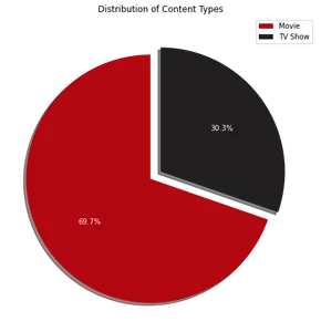
파이 차트 시각화는 Netflix 콘텐츠의 약 70%가 영화로 구성되어 있고 나머지 30%는 TV 프로그램임을 보여줍니다. 다음으로 Netflix가 인기 있는 상위 10개 국가를 식별하기 위해 다음 코드를 사용할 수 있습니다.
Netflix가 인기 있는 상위 10개 국가
다음으로 Netflix가 인기 있는 상위 10개 국가를 식별하기 위해 다음 코드를 사용할 수 있습니다.
# Remove white spaces from 'country' column
df_country['country'] = df_country['country'].str.rstrip() # Find value counts
country_counts = df_country['country'].value_counts() # Select the top 10 countries
top_10_countries = country_counts.head(10) # Plot the top 10 countries
plt.figure(figsize=(16, 10))
colors = ['#b20710'] + ['#221f1f'] * (len(top_10_countries) - 1)
bar_plot = sns.barplot(x=top_10_countries.index, y=top_10_countries.values, palette=colors) plt.xlabel('Country')
plt.ylabel('Number of Titles')
plt.title('Top 10 Countries Where Netflix is Popular') # Add count values on top of each bar
for index, value in enumerate(top_10_countries.values): bar_plot.text(index, value, str(value), ha='center', va='bottom') plt.show()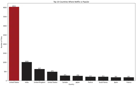
막대 차트 시각화는 미국이 Netflix가 가장 인기 있는 국가임을 나타냅니다.
영화/TV 프로그램 수별 상위 10명의 배우
영화 및 TV 프로그램에 가장 많이 출연한 상위 10명의 배우를 식별하려면 다음 코드를 사용할 수 있습니다.
# Count the occurrences of each actor
cast_counts = df_cast['cast'].value_counts()[1:] # Select the top 10 actors
top_10_cast = cast_counts.head(10) plt.figure(figsize=(16, 8))
colors = ['#b20710'] + ['#221f1f'] * (len(top_10_cast) - 1)
bar_plot = sns.barplot(x=top_10_cast.index, y=top_10_cast.values, palette=colors) plt.xlabel('Actor')
plt.ylabel('Number of Appearances')
plt.title('Top 10 Actors by Movie/TV Show Count') # Add count values on top of each bar
for index, value in enumerate(top_10_cast.values): bar_plot.text(index, value, str(value), ha='center', va='bottom') plt.show()
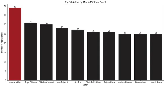
막대 차트는 Anupam Kher가 영화 및 TV 쇼에서 가장 많이 출연했음을 보여줍니다.
영화/TV 프로그램 수 기준 상위 10개 감독
가장 많은 수의 영화 또는 TV 프로그램을 감독한 상위 10명의 감독을 식별하려면 다음 코드를 사용할 수 있습니다.
# Count the occurrences of each actor
director_counts = df_director['director'].value_counts()[1:] # Select the top 10 actors
top_10_directors = director_counts.head(10) plt.figure(figsize=(16, 8))
colors = ['#b20710'] + ['#221f1f'] * (len(top_10_directors) - 1)
bar_plot = sns.barplot(x=top_10_directors.index, y=top_10_directors.values, palette=colors) plt.xlabel('Director')
plt.ylabel('Number of Movies/TV Shows')
plt.title('Top 10 Directors by Movie/TV Show Count') # Add count values on top of each bar
for index, value in enumerate(top_10_directors.values): bar_plot.text(index, value, str(value), ha='center', va='bottom') plt.show()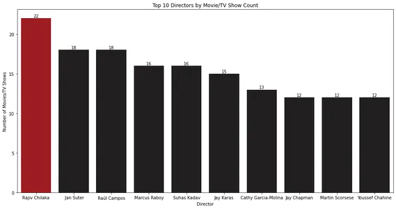
막대 차트는 영화 또는 TV 프로그램이 가장 많은 상위 10명의 감독을 표시합니다. Rajiv Chilaka는 Netflix 라이브러리에서 가장 많은 콘텐츠를 감독한 것으로 보입니다.
영화/TV 프로그램 수별 상위 10개 카테고리
다양한 범주의 콘텐츠 분포를 분석하려면 다음 코드를 사용할 수 있습니다.
df_listed_in['listed_in'] = df_listed_in['listed_in'].str.strip() # Count the occurrences of each actor
listed_in_counts = df_listed_in['listed_in'].value_counts() # Select the top 10 actors
top_10_listed_in = listed_in_counts.head(10) plt.figure(figsize=(12, 8))
bar_plot = sns.barplot(x=top_10_listed_in.index, y=top_10_listed_in.values, palette=colors) # Customize the plot
plt.xlabel('Category')
plt.ylabel('Number of Movies/TV Shows')
plt.title('Top 10 Categories by Movie/TV Show Count')
plt.xticks(rotation=45) # Add count values on top of each bar
for index, value in enumerate(top_10_listed_in.values): bar_plot.text(index, value, str(value), ha='center', va='bottom') # Show the plot
plt.show()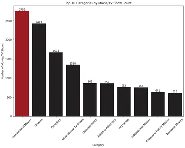
막대형 차트는 영화 및 TV 프로그램의 상위 10개 범주를 개수에 따라 표시합니다. '해외 영화'가 가장 지배적인 카테고리이고 '드라마'가 그 뒤를 잇습니다.
시간이 지남에 따라 추가되는 영화 및 TV 프로그램
시간 경과에 따른 영화 및 TV 프로그램 추가를 분석하려면 다음 코드를 사용할 수 있습니다.
# Filter the DataFrame to include only Movies and TV Shows
df_movies = df[df['type'] == 'Movie']
df_tv_shows = df[df['type'] == 'TV Show'] # Group the data by year and count the number of Movies and TV Shows # added in each year
movies_count = df_movies['year_added'].value_counts().sort_index()
tv_shows_count = df_tv_shows['year_added'].value_counts().sort_index() # Create a line chart to visualize the trends over time
plt.figure(figsize=(16, 8))
plt.plot(movies_count.index, movies_count.values, color='#b20710', label='Movies', linewidth=2)
plt.plot(tv_shows_count.index, tv_shows_count.values, color='#221f1f', label='TV Shows', linewidth=2) # Fill the area under the line charts
plt.fill_between(movies_count.index, movies_count.values, color='#b20710')
plt.fill_between(tv_shows_count.index, tv_shows_count.values, color='#221f1f') # Customize the plot
plt.xlabel('Year')
plt.ylabel('Count')
plt.title('Movies & TV Shows Added Over Time')
plt.legend() # Show the plot
plt.show()
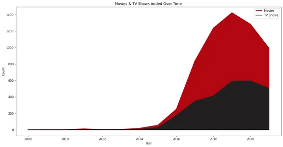
선 차트는 시간 경과에 따라 Netflix에 추가된 영화 및 TV 프로그램의 수를 보여줍니다. 영화와 TV 쇼에 대한 별도의 라인으로 콘텐츠 추가의 성장과 추세를 시각적으로 나타냅니다.
Netflix는 2015년부터 실질적인 성장을 보였고 수년 동안 TV 프로그램보다 영화가 더 많이 추가된 것을 볼 수 있습니다.
또한 2020년에 콘텐츠 추가가 감소한 것도 흥미롭습니다. 이는 팬데믹 상황 때문일 수 있습니다.
다음으로 여러 달에 걸친 콘텐츠 추가 분포를 살펴봅니다. 이 분석은 패턴을 파악하고 Netflix에서 새로운 콘텐츠를 소개하는 시기를 이해하는 데 도움이 됩니다.
월별로 추가된 콘텐츠
이를 조사하기 위해 'date_added' 열에서 월을 추출하고 각 월의 발생 횟수를 계산합니다. 이 데이터를 막대 차트로 시각화하면 콘텐츠 추가가 가장 많은 달을 빠르게 식별할 수 있습니다.
# Extract the month from the 'date_added' column
df['month_added'] = pd.to_datetime(df['date_added']).dt.month_name() # Define the order of the months
month_order = ['January', 'February', 'March', 'April', 'May', 'June', 'July', 'August', 'September', 'October', 'November', 'December'] # Count the number of shows added in each month
monthly_counts = df['month_added'].value_counts().loc[month_order] # Determine the maximum count
max_count = monthly_counts.max() # Set the color for the highest bar and the rest of the bars
colors = ['#b20710' if count == max_count else '#221f1f' for count in monthly_counts] # Create the bar chart
plt.figure(figsize=(16, 8))
bar_plot = sns.barplot(x=monthly_counts.index, y=monthly_counts.values, palette=colors) # Customize the plot
plt.xlabel('Month')
plt.ylabel('Count')
plt.title('Content Added by Month') # Add count values on top of each bar
for index, value in enumerate(monthly_counts.values): bar_plot.text(index, value, str(value), ha='center', va='bottom') # Rotate x-axis labels for better readability
plt.xticks(rotation=45) # Show the plot
plt.show()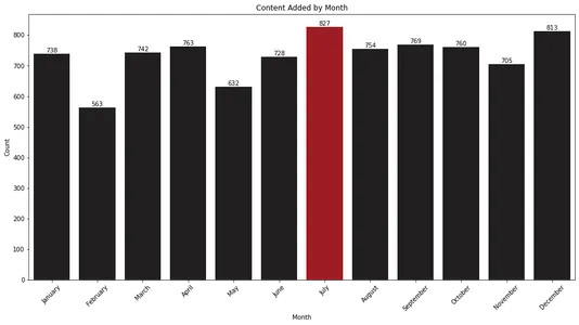
막대 차트는 XNUMX월과 XNUMX월이 Netflix가 라이브러리에 가장 많은 콘텐츠를 추가하는 달임을 보여줍니다. 이 정보는 이 기간 동안 새 릴리스를 예상하려는 시청자에게 유용할 수 있습니다.
Netflix 콘텐츠 분석의 또 다른 중요한 측면은 시청률 분포를 이해하는 것입니다. 각 평가 범주의 수를 조사하여 플랫폼에서 가장 널리 퍼진 콘텐츠 유형을 결정할 수 있습니다.
등급 분포
각 등급 범주의 발생을 계산하는 것으로 시작하여 막대 차트를 사용하여 시각화합니다. 이 시각화는 등급 분포에 대한 명확한 개요를 제공합니다.
# Count the occurrences of each rating
rating_counts = df['rating'].value_counts() # Create a bar chart to visualize the ratings
plt.figure(figsize=(16, 8))
colors = ['#b20710'] + ['#221f1f'] * (len(rating_counts) - 1)
sns.barplot(x=rating_counts.index, y=rating_counts.values, palette=colors) # Customize the plot
plt.xlabel('Rating')
plt.ylabel('Count')
plt.title('Distribution of Ratings') # Rotate x-axis labels for better readability
plt.xticks(rotation=45) # Show the plot
plt.show()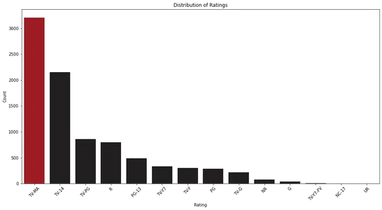
막대 차트를 분석하면 Netflix의 시청률 분포를 관찰할 수 있습니다. 가장 일반적인 등급 범주와 상대적 빈도를 식별하는 데 도움이 됩니다.
장르 상관관계 히트맵
장르는 Netflix에서 콘텐츠를 분류하고 구성하는 데 중요한 역할을 합니다. 장르 간의 상관관계를 분석하면 다양한 유형의 콘텐츠 간의 흥미로운 관계를 파악할 수 있습니다.
장르 상관 관계를 조사하고 XNUMX으로 채우기 위해 장르 데이터 DataFrame을 생성합니다. 원본 DataFrame의 각 행을 반복하여 나열된 장르를 기반으로 장르 데이터 DataFrame을 업데이트합니다. 그런 다음 이 장르 데이터를 사용하여 상관관계 매트릭스를 만들고 히트맵으로 시각화합니다.
# Extracting unique genres from the 'listed_in' column
genres = df['listed_in'].str.split(', ', expand=True).stack().unique() # Create a new DataFrame to store the genre data
genre_data = pd.DataFrame(index=genres, columns=genres, dtype=float) # Fill the genre data DataFrame with zeros
genre_data.fillna(0, inplace=True) # Iterate over each row in the original DataFrame and update the genre data DataFrame
for _, row in df.iterrows(): listed_in = row['listed_in'].split(', ') for genre1 in listed_in: for genre2 in listed_in: genre_data.at[genre1, genre2] += 1 # Create a correlation matrix using the genre data
correlation_matrix = genre_data.corr() # Create the heatmap
plt.figure(figsize=(20, 16))
sns.heatmap(correlation_matrix, annot=False, cmap='coolwarm') # Customize the plot
plt.title('Genre Correlation Heatmap')
plt.xticks(rotation=90)
plt.yticks(rotation=0) # Show the plot
plt.show()
히트맵은 서로 다른 장르 간의 상관관계를 보여줍니다. 히트맵을 분석하면 TV 드라마와 국제 TV 쇼, 로맨틱 TV 쇼, 국제 TV 쇼와 같은 특정 장르 간의 강한 양의 상관관계를 식별할 수 있습니다.
영화 길이 및 TV 쇼 에피소드 수 분포
영화 및 TV 프로그램의 재생 시간을 이해하면 콘텐츠 길이에 대한 통찰력을 얻을 수 있고 시청자가 시청 시간을 계획하는 데 도움이 됩니다. 영화 길이와 TV 프로그램 길이의 분포를 살펴보면 Netflix에서 제공되는 콘텐츠를 더 잘 이해할 수 있습니다.
이를 달성하기 위해 '기간' 열에서 영화 길이와 TV 프로그램 에피소드 수를 추출합니다. 그런 다음 히스토그램과 박스 플롯을 플로팅하여 영화 길이와 TV 프로그램 길이의 분포를 시각화합니다.
# Extract the movie lengths and TV show episode counts
movie_lengths = df_movies['duration'].str.extract('(d+)', expand=False).astype(int)
tv_show_episodes = df_tv_shows['duration'].str.extract('(d+)', expand=False).astype(int) # Plot the histogram
plt.figure(figsize=(10, 6))
plt.hist(movie_lengths, bins=10, color='#b20710', label='Movies')
plt.hist(tv_show_episodes, bins=10, color='#221f1f', label='TV Shows') # Customize the plot
plt.xlabel('Duration/Episode Count')
plt.ylabel('Frequency')
plt.title('Distribution of Movie Lengths and TV Show Episode Counts')
plt.legend() # Show the plot
plt.show()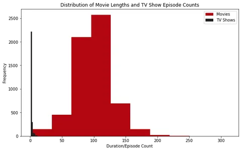
히스토그램을 분석하면 Netflix에 있는 대부분의 영화의 재생 시간이 약 100분임을 알 수 있습니다. 반면 Netflix의 대부분의 TV 프로그램은 한 시즌만 있습니다.
또한 박스 플롯을 검토하면 약 2.5시간보다 긴 영화가 이상치로 간주된다는 것을 알 수 있습니다. TV 프로그램의 경우 사계절이 넘는 프로그램을 찾는 것은 드문 일입니다.
수년에 걸친 영화/TV 쇼 길이의 추세
영화 길이와 TV 쇼 에피소드 수가 수년에 걸쳐 어떻게 발전했는지 이해하기 위해 선 차트를 그릴 수 있습니다. 이러한 추세를 분석하여 콘텐츠 기간의 패턴 또는 변화를 식별합니다.
먼저 '기간' 열에서 영화 길이와 TV 쇼 에피소드 수를 추출합니다. 그런 다음 수년 동안 영화 길이와 TV 쇼 에피소드의 변화를 시각화하기 위해 선 플롯을 만듭니다.
import seaborn as sns
import matplotlib.pyplot as plt # Extract the movie lengths and TV show episodes from the 'duration' column
movie_lengths = df_movies['duration'].str.extract('(d+)', expand=False).astype(int)
tv_show_episodes = df_tv_shows['duration'].str.extract('(d+)', expand=False).astype(int) # Create line plots for movie lengths and TV show episodes
plt.figure(figsize=(16, 8)) plt.subplot(2, 1, 1)
sns.lineplot(data=df_movies, x='release_year', y=movie_lengths, color=colors[0])
plt.xlabel('Release Year')
plt.ylabel('Movie Length')
plt.title('Trend of Movie Lengths Over the Years') plt.subplot(2, 1, 2)
sns.lineplot(data=df_tv_shows, x='release_year', y=tv_show_episodes,color=colors[1])
plt.xlabel('Release Year')
plt.ylabel('TV Show Episodes')
plt.title('Trend of TV Show Episodes Over the Years') # Adjust the layout and spacing
plt.tight_layout() # Show the plots
plt.show()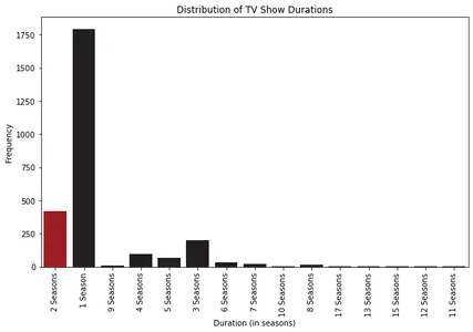
꺾은선형 차트를 분석하면서 흥미로운 패턴을 관찰했습니다. 영화 길이는 처음에는 1963-1964년경까지 증가하다가 점차 감소하여 평균 100분 정도에서 안정화되는 것을 볼 수 있습니다. 이는 시간이 지남에 따라 청중의 선호도가 변하고 있음을 시사합니다.
TV 쇼 에피소드와 관련하여 2000년대 초반부터 넷플릭스의 대부분의 TV 쇼가 XNUMX~XNUMX개의 시즌으로 구성된 일관된 경향을 발견했습니다. 이는 시청자 사이에서 짧은 시리즈 또는 제한된 시리즈 형식에 대한 선호도를 나타냅니다.
제목 및 설명에서 가장 일반적인 단어
제목과 설명에 사용된 가장 일반적인 단어를 분석하면 Netflix의 주제와 콘텐츠에 대한 통찰력을 얻을 수 있습니다. Netflix 콘텐츠의 제목과 설명을 기반으로 이러한 패턴을 발견하기 위해 워드 클라우드를 생성할 수 있습니다.
from wordcloud import WordCloud # Concatenate all the titles into a single string
text = ' '.join(df['title']) wordcloud = WordCloud(width = 800, height = 800, background_color ='white', min_font_size = 10).generate(text) # plot the WordCloud image
plt.figure(figsize = (8, 8), facecolor = None)
plt.imshow(wordcloud)
plt.axis("off")
plt.tight_layout(pad = 0) plt.show() # Concatenate all the titles into a single string
text = ' '.join(df['description']) wordcloud = WordCloud(width = 800, height = 800, background_color ='white', min_font_size = 10).generate(text) # plot the WordCloud image
plt.figure(figsize = (8, 8), facecolor = None)
plt.imshow(wordcloud)
plt.axis("off")
plt.tight_layout(pad = 0) plt.show()
제목의 단어 구름을 살펴보면 "Love", "Girl", "Man", "Life", "World"와 같은 용어가 자주 사용되어 로맨틱, 성장, 드라마의 존재를 나타냅니다. Netflix 콘텐츠 라이브러리의 장르.
설명을 위해 단어 구름을 분석하면 "생명", "찾다", "가족"과 같은 지배적인 단어를 발견하여 Netflix의 콘텐츠에 널리 퍼져 있는 개인적인 여정, 관계 및 가족 역학이라는 주제를 암시합니다.
영화 및 TV 프로그램의 기간 배포
영화 및 TV 프로그램의 길이 분포를 분석하면 Netflix에서 제공되는 콘텐츠의 일반적인 길이를 이해할 수 있습니다. 상자 그림을 만들어 이러한 분포를 시각화하고 이상치 또는 표준 기간을 식별할 수 있습니다.
# Extracting and converting the duration for movies
df_movies['duration'] = df_movies['duration'].str.extract('(d+)', expand=False).astype(int) # Creating a boxplot for movie duration
plt.figure(figsize=(10, 6))
sns.boxplot(data=df_movies, x='type', y='duration')
plt.xlabel('Content Type')
plt.ylabel('Duration')
plt.title('Distribution of Duration for Movies')
plt.show() # Extracting and converting the duration for TV shows
df_tv_shows['duration'] = df_tv_shows['duration'].str.extract('(d+)', expand=False).astype(int) # Creating a boxplot for TV show duration
plt.figure(figsize=(10, 6))
sns.boxplot(data=df_tv_shows, x='type', y='duration')
plt.xlabel('Content Type')
plt.ylabel('Duration')
plt.title('Distribution of Duration for TV Shows')
plt.show()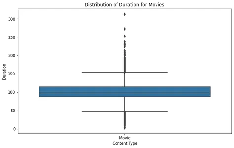
영화 박스 플롯을 분석하면 대부분의 영화가 합리적인 지속 시간 범위 내에 속하고 약 2.5시간을 초과하는 특이치가 거의 없음을 알 수 있습니다. 이것은 Netflix의 대부분의 영화가 표준 시청 시간에 맞게 설계되었음을 시사합니다.
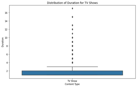
TV 쇼의 경우 박스 플롯은 대부분의 쇼가 XNUMX~XNUMX개의 시즌으로 구성되어 있으며 극소수의 특이치가 더 긴 기간을 갖는다는 것을 보여줍니다. 이는 Netflix가 더 짧은 시리즈 형식에 집중하고 있음을 나타내는 초기 추세와 일치합니다.
결론
이 기사의 도움으로 우리는 다음에 대해 배울 수 있었습니다.
- 수량: 우리의 분석에 따르면 Netflix는 TV 프로그램보다 더 많은 영화를 추가했으며, 이는 영화가 콘텐츠 라이브러리를 지배할 것이라는 기대와 일치합니다.
- 콘텐츠 추가: XNUMX월은 Netflix가 가장 많은 콘텐츠를 추가하는 달로 나타났고, XNUMX월이 근소한 차이로 콘텐츠 출시에 대한 전략적 접근을 나타냅니다.
- 장르 상관관계: TV 드라마와 해외 TV 쇼, 로맨틱 및 국제 TV 쇼, 독립 영화와 드라마 등 다양한 장르 간에 강한 긍정적 연관성이 관찰되었습니다. 이러한 상관 관계는 시청자 선호도 및 콘텐츠 상호 연결에 대한 통찰력을 제공합니다.
- 영화 길이: 영화 길이 분석은 1960년대에 최고조에 달한 후 100분 전후로 안정화되어 시간이 지남에 따라 영화 길이의 추세를 강조합니다.
- TV 쇼 에피소드: Netflix의 대부분의 TV 쇼는 한 시즌으로 구성되어 있어 시청자 사이에서 짧은 시리즈를 선호합니다.
- 일반적인 주제: 사랑, 삶, 가족, 모험과 같은 단어가 제목과 설명에서 자주 발견되어 Netflix 콘텐츠에서 반복되는 주제를 포착했습니다.
- 등급 분포: 수년에 걸친 등급 분포는 진화하는 콘텐츠 환경과 청중 수용에 대한 통찰력을 제공합니다.
- 데이터 기반 인사이트: 데이터 분석 여정은 Netflix 콘텐츠 환경의 미스터리를 풀고 시청자와 콘텐츠 제작자에게 귀중한 인사이트를 제공하는 데이터의 힘을 보여주었습니다.
- 지속적인 관련성: 스트리밍 산업이 발전함에 따라 Netflix와 방대한 라이브러리의 역동적인 환경을 탐색하는 데 이러한 패턴과 추세를 이해하는 것이 점점 더 중요해지고 있습니다.
- 행복한 스트리밍: 이 블로그가 Netflix 세계로의 계몽적이고 즐거운 여행이 되었기를 바라며, 끊임없이 변화하는 콘텐츠 제공에서 매력적인 이야기를 탐색할 것을 권장합니다. 데이터가 스트리밍 모험을 안내하도록 하십시오!
공식 문서 및 리소스
아래에서 분석에 사용된 라이브러리에 대한 공식 링크를 찾으십시오. 이러한 라이브러리에서 제공하는 방법 및 기능에 대한 자세한 내용은 다음 링크를 참조하십시오.
- 판다 : https://pandas.pydata.org/
- 넘파이: https://numpy.org/
- Matplotlib : https://matplotlib.org/
- 사이파이: https://scipy.org/
- 시본: https://seaborn.pydata.org/
이 기사에 표시된 미디어는 Analytics Vidhya의 소유가 아니며 작성자의 재량에 따라 사용됩니다.
관련
- SEO 기반 콘텐츠 및 PR 배포. 오늘 증폭하십시오.
- PlatoAiStream. Web3 데이터 인텔리전스. 지식 증폭. 여기에서 액세스하십시오.
- 미래 만들기 w Adryenn Ashley. 여기에서 액세스하십시오.
- PREIPO®로 PRE-IPO 회사의 주식을 사고 팔 수 있습니다. 여기에서 액세스하십시오.
- 출처: https://www.analyticsvidhya.com/blog/2023/06/netflix-case-study-eda-unveiling-data-driven-strategies-for-streaming/

