_{Figure 1. Partitioning a Dataset into K clusters using K-means and decision trees (IMM & ExKMC) – Source}

IMM Clustering

Iterative Mistake Minimization (IMM) clustering is a tree-based clustering algorithm that builds a decision tree with the same number of leaves as the number of clusters considered in K-means clustering.

The following steps describe how the algorithm works on a high level:

_{Figure 2. A red point moves to the cluster of blue points by the split. This, in IMM clustering, is known as a mistake as the split led to separation of the red point from its original cluster – Source}

Under the hood, the following steps happen while building the decision tree:

• A reference set of K centres from a standard clustering algorithm is obtained for a dataset X.
• Each data point Xj is assigned the label yj based on the centre it is closest to.
• A decision tree is then built top-down using binary splits.
• If a node contains two or more of the reference centres, then it is split again. This is done by picking a feature and a corresponding threshold value such that the resulting split sends at least one reference centre to each side and moreover produces the fewest mistakes: that is, separates the minimum points from their corresponding centres.
• The optimal split is found by scanning through all pairs efficiently by dynamic programming. This node is then added to the tree.
• The tree stops growing where each of the K centres is in its own leaf.

Growing a Bigger Tree – ExKMC Clustering

ExKMC is an extension of IMM where the authors [3] proposed growing the trees, such that the number of leaves exceeds the number of clusters (from K-means), to achieve better partitioning.

• The algorithm intakes a value K, a dataset X, and a number of leaves K’>K.
• ExKMC starts with a set of K reference centers taken from any clustering algorithm. This is followed by building a threshold tree with K leaves (IMM algorithm).
• The best feature-threshold pair to expand the tree one node at a time is computed.
• The tree is expanded by splitting the node with the most improvement to the surrogate cost. Here, the surrogate cost is the sum of squared distances between data points and their closest reference centre (as obtained from K-means).

Given reference centres μ₁,…,μ_k and a threshold tree T that defines the clustering (C¹ ,…..,C^k), the surrogate cost is :

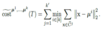
Splitting of a node happens with the combination of a feature and threshold that leads to the most improvement to the surrogate cost.

Implementing in Python

The Python packages for IMM & ExKMC
algorithms are available publicly and can be installed using the following line
of code –

pip install ExKMC

We use the Iris dataset here to analyze how the two algorithms perform in terms of the ‘mistakes’ they produce with respect to the reference K-means clustering.

1) We start with importing the libraries that we need :

from ExKMC.Tree import Tree
from IPython.display import Image

2) We then read the dataset:

df1 = pd.read_csv(r"/content/drive/MyDrive/iris.csv")

3) The tree we build in the next step requires a kmeans model, so we perform the default kmeans clustering.

X = df1.drop('variety',axis=1)
for cols in X.columns:
  X[cols] = X[cols].astype(float)
  k1=X[cols].mean()
  k2 = np.std(X[cols])
  X[cols] = (X[cols] - k1)/k2
k=3
kmeans = KMeans(k,random_state=43)
kmeans.fit(X)
p = kmeans.predict(X)
class_names = np.array(['Setosa', 'Versicolor', 'Virginica'])

4) As per the IMM algorithm, we build the decision tree (that needs the number of clusters that we used in K-means (k) and the K-means model) :

tree = Tree(k=k)
tree.fit(X, kmeans)

5) Next, we plot the tree that we just built using the code below:

tree.plot(filename="test", feature_names=X.columns)
Image(filename='test.gv.png')

Output:

Since the X was scaled before carrying out the clustering, we see some of the thresholds to be negatives in the decision tree.

6) Until now, we have used the IMM algorithm – which is why we got the decision tree with exactly K leaves. In order to have a decision tree with K’ > K leaves, we will use the ExKMC algorithm. To use this, we can pass another parameter called ‘max_leaves’ to our Tree object. This parameter would take the number of leaves (or K’) that we would like to have in our decision tree.

tree = Tree(k=k, max_leaves=6)
tree.fit(X, kmeans)
tree.plot(filename="test", feature_names=X.columns)
Image(filename='test.gv.png')

Output:

As we can see in the above Figure, there are 6 leaves as we passed to the tree object.

Decisioning Through the Trees

We will start by analyzing the output of the tree built by the IMM algorithm.

The first output was from the IMM algorithm with a number of leaves equal to the number of clusters (3). The rules from the created decision tree bring in the explainability ascpect. Due to the inability of the decision tree with 3 leaves to form the same clusters as the K-means clustering, we see some mistakes at the bottom 2 nodes. As mentioned before, mistakes here refer to the points isolated from their reference cluster centre (from K-means) at each node. There, at the left-most bottom leaf, 8 samples belong to some other cluster.

The second output was the ExKMC output which produced a decision tree with 6 leaves. Here, owing to the higher depth of the tree with respect to the decision tree produced by IMM algorithm, we see fewer mistakes at the 6 leaves. As we see in the Table 1 below, there are some splits in the Tree that are redundant for any explanations – e.g. the node at the right bottom with the decision rule – Sepal Length >=1.280.

_{Table 1. Decision Rules For Explaining Each Cluster (From Output of ExKMC algorithm)}

Standard Clustering techniques are difficult to interpret because they cannot pinpoint the reasons behind formation of the clusters. Knowing the rules or boundary conditions that push a data point to a certain cluster can be very insightful for decision-makers. Algorithms that can bring in explainability to clustering are therefore sought after across the industry.

• We looked at two techniques that use decision trees for clustering in order to bring in explainability. The partitions used in the decision tree can be used to explain the creation of the different clusters.
• IMM clustering creates a decision tree with a number of leaves equal to the number of clusters that Kmeans clustering considers.
• For better partitioning, ExKMC is an extension of IMM with more leaves than the number of clusters (from Kmeans).

Connect with me on LinkedIn: Nibedita Dutta

The media shown in this article is not owned by Analytics Vidhya and is used at the Author’s discretion.

Related